
Objective
There is a wide range of applications for Unmanned Aerial Vehicles that have been made possible through recent advancements in technology. One application uses a quadcopter for surveillance of a region. In this project, we attempted to automate a quadcopter for tracking targets. The goal was to have the quadcopter continuously follow and hover directly above the target at a predetermined height.
Introduction
We built an autonomous control system for a drone that tracks and follows an object. Our system is capable of switching control of the drone between the Raspberry Pi and a handheld radio controller as well as switch between hover and autonomous flight where the drone follows a red object below it. The Raspberry Pi 3 is used as the decision making unit to read data from multiple sensors and control outputs from a PWM generating chip to the onboard flight controller using a relay. We successfully integrated the necessary hardware to control the quadcopter and track a target. Additionally, we met the goals we set for ourselves within the scope of the embedded system.
Design and Testing
At the start of the semester, Tim owned a drone he built using parts bought off the internet. His original drone contained a frame, legs, motors, a battery, a radio controller, a radio receiver, a motor controller, and necessary electrical connections between each of the components. The team executed design and testing in a two-pronged approach – Tim and Alex developed the flight controller while Christian worked on computer vision. The flight controller team also developed the overall systems architecture that allows the computer vision and proximity sensor to provide data to the flight controller.
System Architecture
Below is a detailed schematic of the hardware the team developed to connect the Raspberry Pi to the quadcopter’s controller. You can click to enlarge the image.
Hardware
Switching Relays
It is very risky to allow an aircraft to behave autonomously. Although the quadcopter is small, the speed of the blades creates a safety hazard. Furthermore, a “runaway” quadcopter scenario can be dangerous for airplanes in the surrounding area, and is also illegal. Therefore, the team made the first goal of development ensuring it was possible to regain control should the quadcopter begin to fly away. Therefore, a multi-channel relay was used. A relay is a switch controlled by a logic signal. When not energized, the a “normally closed” contact is connected to the “common” contact. Once energized, the switch flips, and a “normally open” contact makes a connection with the “common” contact. This happens mechanically by moving a solenoid against a spring. By connecting the signal from the handheld radio controller to the “normally closed” contact, and the signal from the Raspberry Pi to the “normally open” contact, it is possible to change where control signals are coming from. This also allows the Raspberry Pi to only need to send desired directions – such as “fly forward” – rather than actually calculate and control the dynamics of the quadcopter.
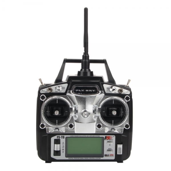
Radio Frequency Controller
The signal to change the state of the relays needed to come from the Raspberry Pi itself, since the handheld radio controller cannot send digital signals that the relay will recognize as a “change state” signal. Luckily, though, Tim’s handheld radio controller sends a 3.3V PWM signal at 50 Hz. Furthermore, the system is set up to send six channels of data, even though there are only four flight commands – roll (strafe left/right), elevation (forward/backward), throttle (up/down), and azimuth (turn). This left two more channels open for other types of inputs, which included any of the four toggle switches on the radio controller.
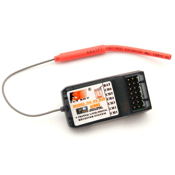
Therefore, the Raspberry Pi can be configured to read those PWM signals from the radio receiver, and use the state of either channel 5 or 6 to toggle the state of the relay. Switch A (channel 5) was chosen to switch from human to computer controlled flight.
It was not just the switches that sent PWM signals from the radio receiver. All six channels outputted a 50 Hz, 3.3V PWM signal which sent signals using duty cycle. This meant the Raspberry Pi also needed to generate the same types of signals. Unfortunately, the Raspberry Pi only has two high-frequency, robust “hardware” PWM pins, and this project needs three highly accurate PWM signals generated at once (the drone cannot autonomously control turning). To that end, the team purchased a “PWM Hat” – a chip that reads serial data signals (encoded with I2C) from the Raspberry Pi, and can generate up to sixteen highly accurate PWM signals without tying up the Pi’s resources or taking the risk of the Linux kernel missing a deadline and crashing the quadcopter.
A quadcopter must have a method of localization in order to execute any sort of autonomous motion. Both a camera and a proximity sensor are used to tell the quadcopter where it is. The proximity sensor uses ultrasonic pulses and the speed of sound to determine distance, while the camera captures colors which are isolated and analyzed to produce a reliable target location using computer vision. Put all together, the control algorithm has a robust error signal on which to base control inputs.
Software
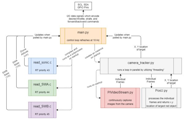
The software for the autonomous quadcopter makes full use of linux’s ability to run parallel processes, as well as the RTOS-like behavior of the Preempt RT kernel patch. The software was integrated according to the following diagram.
Switch Reading
One of the largest hurdles to overcome with the software was reading PWM signals from the radio switches and the time-delay for the ultrasonic rangefinder. First, the PWM signals for the switches left little room for error. The difference between “on” and “off” was a 1 ms and 2 ms pulse (5-10% duty cycle at 50 Hz). Therefore, to ensure proper detection, it is necessary to sample at least once every half a ms (2 kHz). As an added factor of safety, since this reading is keeping the quadcopter from – potentially – flying away, the switches will each be read at 4 kHz. The duty cycle is calculated using the time between a detected rising and falling edge on the pin. The only hardware available on the Raspberry Pi capable of this sort of timing is the nanosecond timer within the C language. Furthermore, python is not able to take full advantage of kernel preemption due to the way the python interpreter works. Preemption is vital for these processes to avoid the computationally intensive image processing from interfering with the deadlines necessary to make accurate readings.
Ultrasonic Rangefinder Reading
The sonic sensor reading process was similar to the switch PWM reading process. The sensor has a range of 4 meters, meaning that sound could take (at 344 m/s in air) up to 0.02326 seconds to make the round trip (8 meters total). The sensor is shown below.
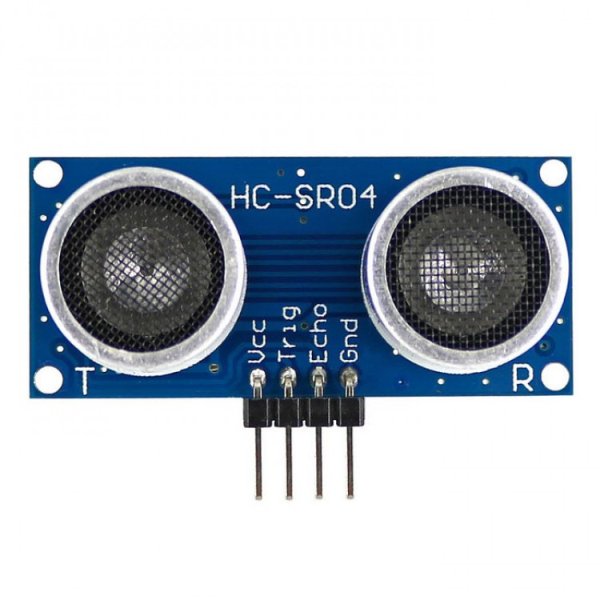
The ultrasonic sensor works by sending a high-pitched sound out out when a logical high value is sent to the “Trig” pin. At that moment, the “Echo” pin is also set high. When the sensor hears the echo of the sonic signal, the “Echo” pin falls to low. The sound has travelled twice the measured distance between the rising and falling edge of “Echo.” Using this information, a high square wave is used to trigger the sensor with a period longer than 0.02326 (shorter than this would cut off distance measurements at the upper end of the sensor’s 4 meter range). Then, the “Echo” pin is polled at a much higher frequency (approx. 13 Khz) to ensure an accurate reading of the actual time delay between trigger and echo. At 13 kHz, the sensor should possess a resolution of approximately 1 cm. An image captured while testing the ultrasonic sensor is shown below.
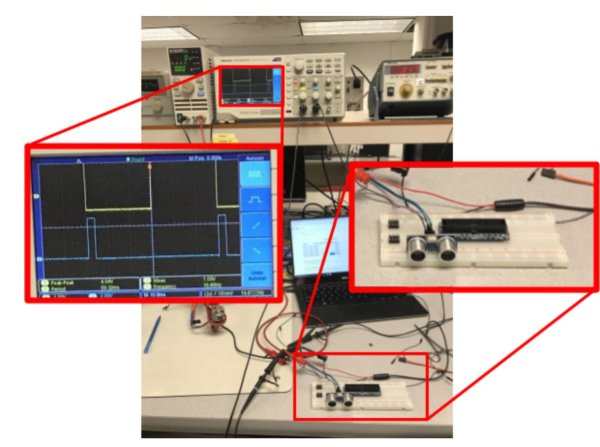
The trigger signal is shown as the top signal on the oscilloscope. The width of the “Echo” response signal in blue on the bottom of the screen changed in proportion to the distance between the sensor and the nearest flat surface.
PWM Generation
Another piece of systems hardware that needed to integrated was the PWM generating circuit. It takes as input a serial I2C data connection through the SDA and SCL pins of the Raspberry Pi. The Arduino python library was immensely helpful with this, and essentially “plug-and-play,” especially with the examples they provide. A link to the development resources on their website is available in the “References” section.
Kernel Optimization
Finally, as the computer vision code was integrated with the rest of the program, the kernel had a tendency to freeze up and die. At first, it would happen every thirty seconds or so. This would only occur when processes were preempting the kernel. So, the RT priorities of the three preempted processes were played with, and their scheduling method was changed from FIFO to RR (round-robin). This seemed to increase time-until-crash to around 3 minutes. At the suggestion of Dr. Skovira, the multi-core architecture of the Raspberry Pi was exploited to keep the computer vision and preempted process separate. First, three of the four cores are reserved using the isolcpus kernel configuration option. This keeps the kernel from scheduling system tasks on any of those cores. Next, the preempted processes are assigned to core 2 using the “taskset” command line tool, and the computer vision processes (and the main control loop) are split across cores 3 and 4. Part of the challenge with this was that the python global interpreter lock which keeps all python processes in the same core. However, several auxiliary (non-python) processes are started, which can be put in another core by playing with the current python process’s core affinity during different start-up tasks. Although difficult to read as a screenshot, below shows the CPU utilization (using htop command) during the execution of the final program. The overall CPU utilization dropped by over 20% after keeping the processes separated on their own cores. Kernel freezing also stopped completely.
Computer Vision
Overview
A goal of the project was to get the drone to track an object and follow it. To do this, we utilized openCV develop a tracking program. The Adafruit PiCamera 2 was used as the camera, and we used the PiCamera library to import the 5 MB RGB picamera image input to a numpy 2D array. Additionally, a video stream script PyVideoStream.py from vision library ‘imutils’ was used run a video stream and output the picamera image frame to be processed. The overall structure of the program architecture can be seen in the ‘Overall software diagram’.
Object Tracking Output
Object tracking is run by a python script, camera_tracking.py. The program contains a single class: tracker. This program updates two states, x and y which correspond to a relative distance in the x and y directions that the drone must move to be centered (relative to the camera center) about the object that is being tracked. Upon creation of the tracking object within main.py, the camera stream is started. Once a method start() is run, an update method is started within a seperate thread. Within this method, the most relevant image frame from the camera stream is accessed, and is passed to a method within the class posU (from PosU.py) to be processed. PosU outputs the desired x and y distances to be traveled by the drone as a percentage.
When running, the the tracker update method loops at 10 Hz. Upon termination of main.py, a method stop() is called which appropriately stops the update thread and initiates the camera stream termination.
Camera Stream
With the start of the tracking program, camera_tracking.py, a PiVideoStream (PiVideoStream.py) object is created. In this class the camera stream is started upon initialization, and the stream resolution, frame rate, and output form is specified. Additionally, a separate thread is started to retrieve the most current frame from the stream as a bgr 2D array and then clear the stream so to save memory space. This current frame is set to an accessible field within the class. The class is set up such that upon termination of the program, a method, stop() can be called to ‘clean up’ the camera process — specifically, shutting down all the processes related to the camera stream. This is important, as these processes will run in the background if not properly shut down, and prevent one from accessing the PiCamera as it can only be used by one process at a time. With this setup, camera_tracker.py can simply pull a frame from the class field whenever a frame is to be processed. The PiVideoStream.py script was originally created by Arian Rosenbrook [1]. This class can also be accessed from the vision library created by Adrian: ‘imutils,’ which can be installed with pip install imutils.
Frame Processing
The object posU, created within camera_tracker.py processes image frames and updates two fields, xdesired and ydesired. By default, if no object is detected, the fields are set to zero such that the drone will not move. For this project, red objects were tracked. The diagram below shows the image processing pipeline when an image frame is passed to posU.
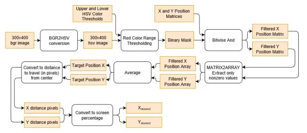
The image is converted to HSV as extracting a color range is easier in this form; to extract red, as we did, we only needed to compare hues. Filtering in HSV also provides the advantage of accounting for fluctuations in lighting and shadows as hue captures the apparent color irrespective of saturation or value.
With a color in mind, we used a trial and error approach to determine the best upper and lower threshold values for extracting red. We specifically calibrated the threshold values to best extract the red of a teammates backpack, so we could us the backpack as the object to be tracked during testing.
With the binary mask created from these thresholds, we considered multiple approaches for determining the object position. At first, we considered extracting the contours of the detected red objects, and then using built in functions within openCV to calculate the moments and subsequent centroid. The problem with this approach is that without filtering out the red picked up from objects that are not being tracked, the object will not be isolated. Additionally, using contours to get the centroid of the red detections gives too much weight to noise and other smaller red objects. Thus, we decided to get the centroid of all the red pixels such that so long as the object desired to be tracked had a large enough concentration of detections by the binary mask, it would decide the centroid.
We examined using morphological transformations to filter out noise and unwanted red detections. Combinations of erosion and dilation could be used to remove small noisy detections, and enhance the larger detections. However, we found using these transformations to not yield significantly different results than when we did not use them. Additionally, using this filtering decreased our processing frame rate from approximately 9 FPS to 4 FPS.
With no filter, we created two position matrices X and Y of the same resolution as an image where a cell corresponding to a pixel location contained either the x pixel location value or y pixel location value. The cells corresponding to non-red pixels were filtered out using a bitwise and operation between the matrix and the mask. Then we approximated the centroid of the object being tracked by averaging each matrix to get an average X and Y location. With the object location known, we easily calculated the pixels to be traveled in the X and Y directions as the target position distance from the center of the camera. To improve the output, xdesired and ydesired should be converted to a unit such as meters.
Interfacing With main.py
Because all of the camera tracking programs were structured as classes, this allowed the main python program, main.py, easily communicate with camera_tracking() by accessing field values from the tracking class and running tracking methods. This is useful for termination of the program, as the main python script can ‘clean up’ the tracking subprocesses through calling a method of the tracking object. all a method within the class to cleanup any opened processes.
Within main.py, to start the object tracking, a tracking object is created, and a the method, start() is run to begin updating xdesired and ydesired. While these two values are automatically updated, they are accessed as needed by the flight controller within main.py via two getter methods. Since the control loop within main.py is within a try-finally statement, when the main.py program shuts down, the stop method within the tracker class is called, and this appropriately stops the frame processing update loop and camera stream.
Flight Control
Additional python code was written in main.py to control the flight of the quadcopter. The first step was to linearize the quadcopter dynamics about hover to make computation easier for the Raspberry Pi. An image detailing the Inertial frame of reference versus the quadcopter’s body and the body frame of reference can be seen below. The full dynamics of the quadcopter in the inertial frame can also be seen below as well as the linearized version of the equations in state space form. Where s is the state of the quadcopter, A and B are the state space matrices, u is the inputs (u1 corresponds to total thrust, u2 corresponds to roll, u3 corresponds to pitch, u4 corresponds to yaw), g is gravity, m is the mass of the quadcopter, L is the lever, or distance from the motor to the quadcopter’s center of gravity, and the I terms are the moments of inertia for each respective axis.
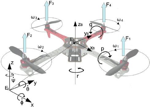
Additionally, the motion of the quadcopter and the x, y, and z position were decoupled and further simplified to decrease computation time. The equations can be seen below.
The optimal control theory LQR (Linear Quadratic Regulator) was chosen to be the controller for the three states. LQR works by solving for an optimal gain matrix K that will be used in full state feedback to drive a state error to zero. The equation can be seen below. Where e is the error state, A and B are the A and B matrices for the x, y and z states individually and K is the optimal gain matrix.
To determine K, first, a cost function was developed and can be seen in the equation below where s is the state of the quadcopter, u is the input, and Q and R are weighting terms. The matrix Q relates to the importance of the quadcopter being at the desired state and the matrix R is related to the how much energy is used by the input of the quadcopter to get to the desired state. Equal weight was set on both terms by setting Q to a 12×12 identity matrix and R to a 4×4 Identity Matrix. Next, the LQR tool in Matlab was used to solve for the optimal gain matrix K in the full state feedback equation seen below. K was determined to be [1 2.43].
To use LQR practically for our application, the inputs into the full state feedback equation had to be extracted then fed into our controller in order to control the quadcopter. The inputs are given by the equation u = Ke. Specifically for height control, since it was stabilized around hover, the height throttle input was added to a “hover throttle” we determined experimentally. The x and y inputs were unaltered.
The equations for full state feedback were then input into main.py. The ultrasonic sensor was used for height feedback and the camera was used for x and y position feedback. A timing function was used to determine the velocity of the quadcopter in each direction by dividing the change in state at each iteration and dividing by the time that elapsed. This was used for obtaining the first time derivative of each state.
Kernel Optimization
Finally, as the computer vision code was integrated with the rest of the program, the kernel had a tendency to freeze up and die. At first, it would happen every thirty seconds or so. This would only occur when processes were preempting the kernel. So, the RT priorities of the three preempted processes were played with, and their scheduling method was changed from FIFO to RR (round-robin). This seemed to increase time-until-crash to around 3 minutes. At the suggestion of Dr. Skovira, the multi-core architecture of the Raspberry Pi was exploited to keep the computer vision and preempted process separate. First, three of the four cores are reserved using the isolcpus kernel configuration option. This keeps the kernel from scheduling system tasks on any of those cores. Next, the preempted processes are assigned to core 2 using the “taskset” command line tool, and the computer vision processes (and the main control loop) are split across cores 3 and 4. Part of the challenge with this was that the python global interpreter lock which keeps all python processes in the same core. However, several auxiliary (non-python) processes are started, which can be put in another core by playing with the current python process’s core affinity during different start-up tasks.
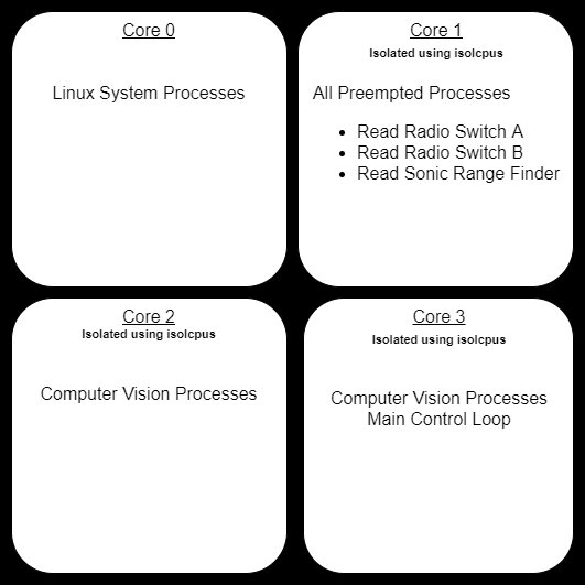
The overall CPU utilization dropped by over 20% after keeping the processes separated on their own cores. Kernel freezing also stopped completely.
Results
Financial
One of the stated goals of the project was to keep all purchased components below $100 total. Because the Raspberry Pi and drone were already in our possession, we did not have to count those toward the $100 limit. Our final budget is as folllows:
| Component | Quantity | Cost |
|---|---|---|
| PiCamera | 1 | $22.00 |
| Geere 4CH 12V Relays | 1 | $12.21 |
| 5V Cell Phone Charger | 1 | $15.00 |
| XT60 Power Cable Splitte | 1 | $3.45 |
| HC-SR04 Sonic Range Finder | 1 | $4.30 |
| Adafruit PWM Generator Chip | 1 | $15.49 |
| Cylewet Bi-Directional Logic Shifter | 1 | $1.10 |
| Total | $73.54 |
At $73.54 total, the project is $26.46 under budget.
Flight Tests and Controller Performance
In order to ensure that the tests were conducted safely and the drone did not fly away out of control, the quadcopter was taken to the nearby baseball field and secured to second base using parachute cord.
Most of the flight tests ended in catastrophic failure. Many parts were broken during this process. Most commonly broken items were propellers and legs of the quadcopter. Sometimes wires would be ripped out and hardware would be violently thrown from the quadcopter.
The initial flight tests were us manually trying to fly the quadcopter. Since when the quadcopter was built it had large ambitions of being able to carry heavy loads, the motors were highly overpowered which made the controls extremely sensitive and hard to control.
The next sequence of flight tests involved finding a throttle to use as a setpoint for the hoverlock feature. For these tests, the throttle was set to a constant in the main.py function and the flight of the quadcopter was observed. When close to what we presumed would be hover, the quadcopter would bob up and down. We consulted with a local expert, student Adam Weld, and he said this is potentially a normal phenomena. The hover throttle we found was then included in the controller calculations.
When tested in the lab, the controller seemed to perform exactly as expected. However, when implemented in actual flight tests, many errors occurred. The quadcopter did not perform at all how expected. To speculate on why the quadcopter did not perform as well during testing, it could potentially have been that the feedback it was receiving from the ultrasonic sensor was inaccurate.
Initially, the gains seemed to be way too high so they were reduced drastically. There was one test where the controller seemed to be working well but on a terrible time delay.
We had the misfortune of burning up a motor. So all four motors were replaced with ones of a lower kv rating which translates to revolutions per applied volts. The quadcopter became easier to fly manually however, this did not seem to solve our issues with autonomous flight.
To eliminate potential errors with obtaining the time derivatives from dividing the difference in heights between control inputs, a simpler proportional controller was implemented and tested. The results were worse. The quadcopter wanted to fly as fast as it could away from its initial location.
It’s hard to troubleshoot what the differences in conditions are when the drone is flying versus when it’s in the lab. One potential source of error could have been that the quadcopter was moving too quickly for the ultrasonic sensor’s update rate and was acting on old height data indicating it was still on the ground when in reality it was a few meters in the air. Additionally, the vibrations that occur during flight could have been disrupting some of the hardware, making it perform differently than in the lab.
Conclusion
This project was a great introduction to independent development on an embedded system. The class labs taught skills needed to navigate the Linux environment, but the final project motivated the design thinking necessary to succeed with embedded systems. All coming from mechanical engineering backgrounds, the team members also learned a great deal about circuits and electrical design. Although flight tests were never strictly a success, they were the types of failures that shed light on the weaknesses of the system.
Future Work
The work accomplished in this project demonstrates that a Raspberry Pi controlled quadcopter is possible. However, the project struggled with testing, especially when the quadcopter itself is difficult to control just using the radio controller. Future work would start with developing a better body for the quadcopter that could centralize the electronic hardware, protect it and dampen the vibrations produced during flight. Additionally, a better testing rig that constrains the quadcopter between two heights so that it cannot crash into the ground would be desirable. Another testing method we were unable to implement due to time constraints would be to have the main.py continuously write to a .csv file with information during flight so that it could be analyzed after a flight to find out what was going on.
Code Appendix
References
Preempt-RT Kernel
blink_v6.c code from Lab 4 in ECE 5725
Adafruit PWM Hat
iscolcpus reference
PiVideoStream.py Reference Using Camera
Changing Color Spaces
Color detection
bitwise_and
Using Contours
OpenCV Documentation
imutils
Read more: Autonomous Quadcopter for Target Tracking