
1 Introduction
As our connection to the internet becomes increasingly important and as new forms of dispens- ing internet services emerge, it is important to identify weak-spots in any internet network. We propose developing Raspberry Pi devices which will continuously monitor the strength of a WiFi signal (Eduroam in our case) and output the values to a web application to continuously update a heatmap. As the devices move around campus, the heatmap will then show areas of weak and strong coverage.
We can imagine a system where multiple people, at different points around Swarthmore, roam the campus and provide valuable data to students, professors, and network engineers on the current state of Eduroam. This will allow everyone to identify the exact location of dead spots or areas of weak coverage. We hope that the final system can be used for identifying weak spots on larger scale networks like LTE or satellite based internet services.
We will rely on common signal strength measurements like Received Signal Strength Indi- cator (RSSI) to quantitatively represent different areas on campus. These can be outputted with the linux module iw. We will also obtain locations for these readings with the GPS module at- tached to our Pi. All readings will have associated degrees of confidence that can be improved over time.
This is an interesting problem to solve because of how it applies many engineering disci- plines to tackle a common issue. We would be using knowledge of networks, hardware-design, probabilistic models, and software engineering principles to approach this task.
The project can be broken down into two major components. The first revolves around the Raspberry Pi and its associated hardware extensions. The Pi handles all of the data collection. The second component relates to our server, which processes all of the data and ultimately serves a web page to the user, displaying all of the information about the current state of the wireless network in question.
2 Raspberry Pi
Our choice for processing inputs was a Raspberry Pi 3B+, running the latest version of Rasp- bian OS. This is a Unix-like OS, giving us the full functionality of a UNIX command line.
2.1 GPS
In order to keep track of our location, we purchased an Adafruit Ultimate GPS Breakout mod- ule which outputs latitude, longitude, and altitude with a 10Hz update frequency. This GPS module was connected to the Pi via a USB Serial connection. The GPS module can be seen in figure 1. Four pins on the GPS were wired to the Pi: TX, RX, GND, and VIN.
Originally, this GPS module was not en- tirely accurate, giving an error of over 30 me- ters. In order to remedy this, an additional antenna was purchased for the GPS unit, in- creasing the rate at which it fixed to satel- lites and improving indoor and outdoor pre- cision.

2.2 Wireless Monitoring
Across most UNIX distros, the iw command
comes pre-installed. This is a new command line utility for wireless devices. This command often gets confused with iwconfig, a now deprecated tool. The new iw utility handles newer generations networking protocols. The commmand that we run on our Pi is
iw dev wlan0 scan
The command invokes the iw utility with the first word. The second word, dev, stands for device. The third word, wlan0, specifies which device we want to look at. In most modern machines, wlan0 refers to the integrated networking card. The last word, scan, looks at all the available networks and outputs their details.
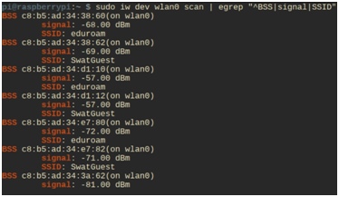
The output of this command is all the wireless networks the Pi can pick up and all of its associated metadata. The only information we are interested in are the SSIDs, MAC addresses, and signal strengths. So we filter the results by those fields with the following extension to our original command:
iw dev wlan0 scan | egrep “∧BSS|Signal|SSID”
2.3 Handling the Data
The entirety of the data collection is done in one Python script, which handles the GPS and WiFi data. The GPS data is obtained with a library known as AGPS3. Originally, we used the library associated with Adafruit; however, we quickly ran into an issue where a backlog of older GPS readings were being saved. This was solved in the newer library with threading. Threading is a tactic employed by programmers to speed up computation for a single process. This new library had threads that handled clearing the old buffer that accumulated overtime. Once the GPS data was streaming in real time, we incorporated the WiFi data previously mentioned. In order to run the shell command in Python, we utilized a builtin library called subprocess. This enables us to run these shell commands as processes from Python and col- lect their output. Thus, for every iteration that we grab a GPS reading, we also run the shell
command and obtain the associated WiFi data.
2.4 JSON Format
After obtaining the GPS and WiFi data every iteration, we must parse through the data, ensure it’s properly formatted and free of errors, and package it into a readable format. The format we chose was a JSON file. JSON format is the industry standard for transferring data between web applications and servers, storing the data as readable tree of nested dictionaries and lists. As we traverse around campus and gather data, our JSON file will continue to grow, eventually reaching over 100,000 lines. This occurs because in addition to saving data for Eduroam, we also hold the data for SwatGuest and SwatDevice. This was a design choice, should we choose to extend our project to other SSIDs as well.
In order to handle random bugs and program interruptions, we have a fail-safe protocol: every 100 iterations, we will save the current copy of our JSON data. Once we have finished all of the data collection, the Python script will push the final JSON file to our AWS server.
2.5 Additional Hardware
While traversing campus, we required a constant source of power to keep the Raspberry Pi running. We purchased an additional battery pack from the official Adafruit site. The choice of battery pack is important because the Raspberry Pi may run into undervoltage issues if not provided a consistent 5V source. Additionally, the cable to power our Pi must be as short as possible, since longer cables tend to have a higher resistance.
Furthermore, an additional touchscreen monitor was purchased to monitor the output of the program on the go.
3 Lightsail Server
3.1 Cloud
In order to serve our desired product to the end-user, we must have a place where we can perform the computationally intensive task of producing the heatmap and hosting our web- site files. Cloud based storage is becoming an increasingly popular choice for consumers and companies to store data. As opposed to traditional storage methods which involve owning large racks of hard-disks on site, cloud storage takes away local storage and hosts your data in a remote location with an easy, intuitive way to interact with it.
The cloud provider we chose for our project is Amazon and their AWS services. AWS offers numerous amounts of services for different needs. However, we opted for a service called Lightsail, which can simply be thought of as a remote computer. Lightsail gives us access to an always-on computer in one of Amazon’s facilities in Virginia, providing us with 16 GBs of RAM, 4 vCPUs, and 320 GBs of flash storage. The computer is running Ubuntu 18.04 as its operating system. Our cloud instance has the static IP address:
18.206.136.194
3.2 Map Generation Theory
Before we get into the Python scripts running on the server, let’s talk about the theory behind our heatmap generation. Recall that after our Pi compiles all of the data into a JSON format, it’s pushed onto our server for further processing. The JSON file contains hundreds of points, each characterized by a latitude, longitude, and a list of all the wireless networks seen by the Pi at that point.
Since we are gathering data across campus, it is impossible to get the signal strength at ev- ery possible latitude and longitude. As such, we are confronted with the problem of estimating the strength at points we don’t have data for. This motivates a need for an interpolation-based approach.
For interpolation, we use a locally weighted regression. We center a 3-dimensional Gaus- sian distribution on each measured point. The distribution values represent how much weight each measurement contributes to the prediction of another point. For every point we are trying to predict, we will use these weights to take a weighted average of measured values. As ex- pected, points near a measured point will be more likely to reflect that point’s measured value than points further away. We can think of the Gaussian distributions as confidence intervals over each point.
To formalize, the distribution that belongs to a particular measurement at point µ will be defined by f:f ∼ N(µ, σ2)
where σ2 is some constant we define and represents the size of the confidence interval for each measurement.
At some other point j, we can then interpolate a value by utilizing all our measured points.
valuej =
| ∑ |
i=1 n
∑n
weights ∗ fi weights
(2)
i=1
where i ∈ S, the set of all measured points.
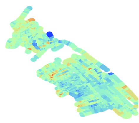
We can populate an entire map of the region of interest with values using this interpolation map. We decide which values to populate by using a grid-based approach. We color-code our map to visually reflect the signal strengths we see.
3.3 Data Processing
Our JSON file is composed of longitude/latitude values. These are not intuitive or relatable units. Ultimately, our map generation algorithm relies on parameters like σ, which represents distance. To better understand and vary such parameters, it is helpful to have all our coordi- nates in meters. Additionally, since the differences between GPS values depend on where you are on earth, parameters like σ would need to vary based on your location too. Because of this, we chose to convert all latitude and longitude values to the Universal Transverse Mercator Co- ordinate System, which is measured in meters and is spatially-consistent regardless of where you are on earth. Python has a utm library which facilitates this unit conversion.
3.4 Image Generation
The image generation is governed by one main Python script. This script reads in the JSON file pushed from the Pi, isolates the SSIDs we want to focus on (Eduroam in our case), converts GPS coordinates to UTM coordinates, and generates a heatmap based on the theory presented earlier. To build our main map, we select Eduroam signals that are the strongest at each point. We then populate the map by following the map generation algorithm at each square in a pre- defined grid. The squares of the grid represent the individual pixels that our algorithm will eventually output.
Once we have populated our grid with values, we have to map the values to intuitive colors. To do this, we normalize our values so that they are all between 0 and 1. Then, we obtain pixel values for our red, green, and blue values by applying a sinusoid function with changing parameters for each color as shown in equation 3. We made the sinusoid for the red-values peak at 1, the sinusoid for the blue-values peak at 0, and the the sinusoid for the green-values peak at 1/2.
a + b ∗ cos(2 ∗ π ∗ (c ∗ val + d))) (3)
3.5 Python Script Optimization
The calculations for the locally weighted regression are time and memory intensive. Since we determine every single measurement’s contribution to each point in our grid, our run-time is
O(lwn). l is the number of rows in our grid, w is the number of columns in our grid, and n is
the number of entries from our JSON file.
Normally, we would execute this in python via three nested “for” loops. To speed up our code, we relied on the numpy library in python which allowed us to use C-based code and matrix operations. We used the meshgrid command to build a matrix for our grid and built another matrix for our measurements. By multiplying the matrices together with broadcasting, we were able to create a three-dimensional “weights” matrix which had dimensions l ∗ w ∗ n. We could then produce the desired results by using a sum function along the second axis. This vectorization sped up our code significantly, but we soon realized that we would run into memory errors if the size of the “weights” matrix grew too large. Because of this, we performed our calculations on small portions of the grid and created smaller “weights” matrices. We would delete each “weights” matrix once it produced the desired results. This process is called “chunking”.
3.6 MAC Address-Based Heatmap
One topic we wanted to explore is localization based on signal strength. To begin to solve this problem we isolated the strength of specific routers. We saw that signal strength tends to taper off as we move away from a router. This understanding could help us build probabilistic models to discover where routers are and, following that, where we are. In future work, we would like to analyze these visualizations more closely.

3.7 Web Development
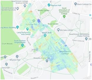
Upon the completion of the image generation, we obtain a PNG image to be overlaid over a map of Swarthmore. In order to present this data to the public, we opted to create a web application on our AWS server. The website consists of three basic files: HTML, CSS, JS. The HTML file is what is rendered on the user’s browser. The CSS file helps with aligning the objects on the site. And finally, the JS file handles the communication with Google to obtain a map of Swarthmore and ultimately overlays the PNG image over it.
3.8 Google Maps API
To display Google’s map on our site, we must communicate with the API that Google Maps provides. The term API defines a set of functions that are provided to us in order to access Google’s features. So in our case, we reference Google Map’s library in our HTML code by providing a private key, allowing us to render their map. The reference to Google Maps in our HTML code can be seen below:
<script src=”https://maps.googleapis.com/maps/api/js?key=<KEY-HERE>
&libraries=visualization”></script>
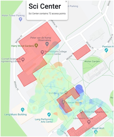
Upon rendering the map, we must overlay the image generated with the Python code. This is done through a series of custom overlay functions provided by Google’s OverlayView class. These functions allow us to manually customize <div> elements in our HTML code, which we define to render the map and custom overlay. Additionally, our map shows some additional information for some buildings, which we outlined with red polygons. These polygons are defined with Google’s Polygon class. Upon a mouse hover event, an InfoWindow appears, informing the user how many routers are in that building.
3.9 Hosting Files with Node JS
In order to serve all the website to the end user, we must have a continuously running web server on our Lightsail instance. Our web server of choice was NodeJS, a popular standard across many industries. At the core of it, NodeJS, when given a directory, automatically pushes the webpage to the user, handling all of the HTML headers and data payload processing for us. By default, it looks for a file named index.html to display on the browser. We additionally specify a port to forward the site to in our configuration file. In our case, Lightsail has ports 22, 80, 8000 open, so we choose 80.
4 Results
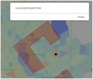
We were able to successfully produce a heat-map and overlay it on Google Maps. We also were able to implement several additional features such as filtering by a single MAC address, click- ing on a point in the map to view its associated signal strength, and hovering over buildings to display the number of routers. . Our site is currently running at:
5 Future Work
In the future, we would like to extend this project to use multiple Pi’s that potentially com- municate with each other. We would also like to add some optimizations that make it usable for large scale networks like LTE. Additionally, we would like to continue exploring the local- ization problem and see if we can obtain a solution that increases the spatial accuracy of our map.
6 Appendix
Note: JavaScript and HTML code not included in Appendices.Python Code on Raspberry Pi
6.1 Python Code on Raspberry Pi
from gps3.agps3threaded import AGPS3mechanism import os
import time import sys import json import subprocess
def getWifi():
command =’sudo iw dev wlan0 scan | egrep “^BSS|signal|SSID”’ while(True):
try:
result = subprocess.check_output(command, shell=True) break
except:
continue
result = str(result)[2::].replace(’(on wlan0)’,””) result = result.replace(’\\n’,’ ’)
result = result.replace(’\\t’,’’).replace(’dBm’, ’’).replace(’SSID:’,’’).replace(’BSS’,’’). replace(’signal:’,’’)
result = result.split()[:-1] tempDict = {}
wifiList = [] prevKey = ’’ i = 0 # MAC Address is key. Value is [dBm,SSId] whilei <len(result)-2:
if (result[i].count(’:’) == 5):
33 if tempDict:
34 wifiList.append(tempDict)
35 tempDict = {}
36 tempDict[’MAC’] = result[i]
37 tempDict[’DBM’] = result[i+1]
39 i += 3
else:
tempDict[’SSID’] += ’ ’ + result[i]
i += 1
return wifiList
49 if name == ’ main ’:
agps_thread = AGPS3mechanism()# Instantiate AGPS3 Mechanisms
agps_thread.stream_data() # From localhost (), or other hosts, by example, (host=’gps.ddns
.net’)
agps_thread.run_thread() # Throttle time to sleep after an empty lookup, default ’()’ 0.2 two tenths of a second
outerDict = {“JsonData”:[]}
i = 0
while 1:
temp = agps_thread.data_stream
data = {}
data[“wifi”] = getWifi()
data[’Latitude’] = temp.lat
data[’Longitude’] = temp.lon
data[’Altitude’] = temp.alt
print(“Iteration : d s s” (i, data[’Latitude’], data[’Longitude’]))
i += 1
outerDict[“JsonData”].append(data)
if (i 100 == 0):
print(“Dumping s” (str(i)))
name = str(i) + ’_wifi_gps_data.json’
with open(name,’w’) as outfile:
json.dump(outerDict, outfile, indent=4)
print(“Written!”)
Source: Live RSSI Mapping System