
1 Introduction
This documentation catalogs the progress made so far in the installation of the Node-Red development tool used for data collection and analysis of Margherita 1 & 2. Not all methods and tools listed are used in the the current finished product, but were listed here in case any future user of Node-RED finds them useful. If you have a new Raspberry Pi and are having trouble setting up the device to begin with, refer to Appendix A for instructions.
1.1 Install Node-RED
To install Node-RED into to a Raspberry Pi, type this specific into the terminal: 1 bash <( curl -sL https :// raw . githubusercontent .com /node – red / raspbian -deb – package / master / resources / update – nodejs -and – nodered ) and press enter. To install Node-RED into a machine that runs Unix/Linux then do the following sudo commmand in the devices terminal: 1 sudo npm install -g –unsafe – perm node – red If you are still having issues, refer to the installation website here: https://nodered.org/docs/gettingstarted/installation
1.2 Base Diagram
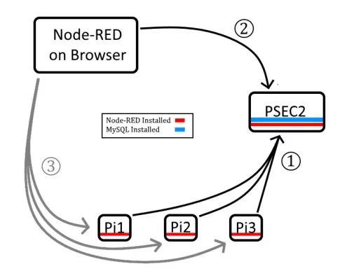
Figure 1 shows an outline of the current possible configurations. With 1 , the data collected by
the Pis directly get sent to a MySQL database in PSEC2 via a Python program. In 2 you open a
browser in your personal computer and point it at PSEC2 via Node-RED. Here, you can implement
programs that can access the data in MySQL and many other important functions which will be
said more in detail later. 3 is a separate option to replace 1 , which is why it’s gray colored,
not black. In 3 you point your personal computer to any of the Pis. Each Pi will have it’s owned
Node-RED on separate tabs if you wish to run more than one. Here, you can create programs
that gets data held in the Pi’s memory and sends it to a MySQL database on PSEC2. This way
is a bit slower but may be easier to fix due to Node-RED’s interface. However, it requires more
steps to set up and contains more moving pieces, which makes it slower and possibly a bit more
frustrating to work. We recommend 1 which doesn’t require the Pis to have Node-RED but you
can use whichever method you find more appropriate. Whether you use 1 or 3 , the 2 step is
the same process.
1.3 Future Structure
For the following subsections, they will specify on which device to work on.
• For anything involving Node-RED on a browser, but not specifically on PSEC2 or a Pi, the
subsection will be accompanied with NR
• For use of Node-RED hosted by PSEC2 the subsection will be accompanied by NRPS
• For use of Node-RED hosted by a Pi the subsection will be accompanied by NRPi
• For use of PSEC2 either by ssh or directly by the terminal of PSEC2 the subsection will be
accompanied by PSEC
2 Node-RED Flows
2.1 Nodes – NR
Nodes are fixed functions that do specific tasks in Node Red. Some Nodes have very specific tasks,
while other Nodes can be manipulated and altered which allows for flexibility. Nodes can act as
the input, output, or bridge in a flow, we’ll speak about flows shortly. You can see Nodes as the
functions in a Python, Java, etc. program/script. Your collection of Nodes can be seen as a toolkit.
To access specific Nodes, check the sidebar to the left in the figure below.
node to another through lines. Together, lines and Nodes constitute a program flow.
You can install more Nodes with the tab at the top right and going to the ’Manage palette’
subsection. Here you can check what Node packages you have installed and can also search up new
Node packages that you may want to install. As a tip, always consult google first for what nodes
you may be looking for before installing.
2.2 Flows – NR
A collection of connected nodes is called a Flow. Flows are essentially the ’program’ you can run,
but without real script. Instead, you have a browser based ’flow’ of functions. You double-click
on each Node to see what they do can do to the Flow. By double-clicking a Node you can also
change the Node’s name, actions, and other special instructions you may want to give the Node.
To compile/run the Flow, click on ’Deploy’, errors will pop up if anything is incorrect with syntax,
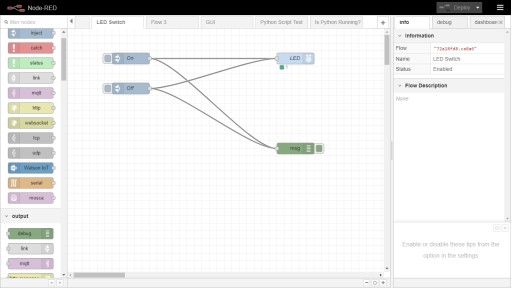
and if no errors appear it will run. Take a look at Figure 3 to see an example of a simple node.
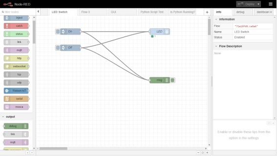
There are two inject nodes, which we labeled ’On’ and ’Off’, that send the string values ’1’
and ’0’ respectively. They both flow into a Pi GPIO Pin output Node (labeled LED) and a Debug
Node. In the GPIO PIN Node, we set which GPIO PIN we want to focus on, for this example
we’ll choose pin 11 GPIO17. We set the default voltage to the value 0, meaning it starts out in
the ’Off’ position. We then deploy our Flow. To turn our LED on, which should be hooked up
to a ground pin and pin 11, we click on the little blue button attached to the left side of ’On’
injector. The LED should then light up. To turn off the LED, we simply click on the button for
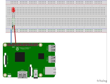
the ’Off’ injector. For reference on the general set up of the wires, resistor and so forth please refer
to Figure 4.
2.3 Debug Node – NR
On the right side of the Flow on Figure 3 you can see a green Node named the Debug Node. The
Debug Node is a useful tool to use while making Flows and is very simple to utilize. On the left
sidebar of the Node-RED, just click and a drag a Debug Node to the main canvas. There, you can
see that it only takes an input, and has no explicit outputs. However, the Debug Node allows to
see what messages are being sent to it directly. To see said messages, you click on the ’debug’ tab
on the right sidebar. There, you see all outputs directed towards the Debug Node input. You can
also specify what part of the data you’d like to see on the ’debug’ window by double-clicking on
the debugger and setting your preferences. I suggest using the ’complete msg object’ option due
to its better descriptions of objects. The Debug Node will tell you what objects are in a message,
what are in those objects, and will tell you errors in a message. The debug tab will also prompt
specific errors coming from any point of the Flow, regardless if there is a Debug Node in the Flow
or not.
3 MySQL Database
Before we begin to do any sort of work in creating the Flow we want, we need to discuss how to
work with MySQL. MySQL was installed by Mary Heintz, so we do not have the steps on how to
install the software into a device.
3.1 Running MySQL – PSEC
In order to start MySQL, you must first open up your ssh client to PSEC2 and type the following
lines. The expressions in parentheses are not commands, just side remarks.
- ssh [email protected]
- mysql -u -p
(Note: if prompted for a password, enter the corrected listed password created by Mary) - show databases;
(Shows you the databases) - use test;
(Opens up the database named ’test’). - show tables;
(Shows you tables within the database you’re in)
3.2 The Table Set Up – PSEC
For the Node-RED flows to work at its current state, the columns of tables should follow the format
in figure 5
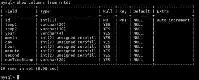
This table is named rnts, random-number-time-stamp, and has an ’id’ column which is the
primary key of this table. Every single instance of data will have a unique id value since it auto
increments (newest values will have the greatest id values). Following the ’id’ column are the
two data columns (temp1 and temp2) with random temperatures ranging from 0 to 20. When
making a real data table to store temperature readings, the number of columns should be the
number of channels which read temperature. The other columns are: year, month, day, hour,
minute, and second, which correspond to the time when the data value was measured. All of these
columns are padded with leading zeros if ever needed (e.g. July is the value ’07’ not ’7’ in the
month column). In the final column we attached all date values together in their column order
and named it ’numTimeStamp’ for numeric time stamp. We have the data as such so we avoid
some extra, unnecessary loops later on in Node-RED.
3.3 Creating a table in MySQL – PSEC
We will be demonstrating how to create a sample table named ’rnts’ in our ’test’ database, just
like in our example. This table will store data from 2 temperature channels (which we denote as
temp1, temp2). Type the following commands into MySQL.
- use test;
- create table sampletable (
id INT NOT NULL AUTO_INCREMENT PRIMARY KEY,
temp1 VARCHAR(20) NOT NULL,
temp2 VARCHAR(20) NOT NULL,
year VARCHAR(4),
month INT(2) ZEROFILL,
day INT(2) ZEROFILL,
hour INT(2) ZEROFILL,
minute INT(2) ZEROFILL,
second INT(2) ZEROFILL,
numTimeStamp INT);
We start each argument on a new line to make the command easier to see. The type VARCHAR
is just a string type and the type INT is an integer type where the following number within
parentheses is the max amount of characters allowed. NOT NULL refers to not allowing the
column to be empty, or have a NULL value. ZEROFILLING is the padding of zeros, which was
referenced in Section 3.2. If you want both commands NOT NULL and ZEROFILL, ZEROFILL
must be typed first given the syntax of MySQL.
3.4 Setting Up MySQL in Node-RED – NRPS & NRPi
The MySQL Node is not pre-installed to Node-RED. To install, you can install with the following
command in a pi’s terminal:
$npm install mysql
$npm install mysqljs/mysql
The first line is to install, the second line is if it states you have to install the latest version from
GitHub. Alternatively, you can also install from the Node-RED interface. You can find Nodes on
a google search, in this case it’s called ’node-red-node-mysql’. Make sure you remembered/copied
the name of the Node then go to the top right tab that looks like 3 horizontal stripes then:
- click on ’manage palette’
- click on the ’Install’ tab
- type the name of said Node
- once you find the Node you want, click install
Once installed, drag and drop a MySQL Node onto the canvas and double click it. It should look
like Figure 6.
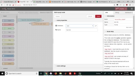
Here, the Database section will be empty. Add a new MySQL Database. For now, our Database
is titled ’test’. Be mindful that this name must be the same as the database you would like to
push/pull data from. Then, you add other details about the MySQL Database, shown in Figure 7.
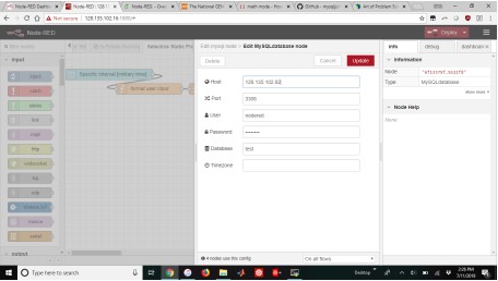
Here you specify the IP Address of the device that hosts the MySQL Database. You keep the
port as is (3306). Be sure to grant privileges to your device so that it can access to MySQL by
granting a username and password access, we did this through Mary Heintz. You then have to
put this username and password of the device Node-RED is running on. Then input the Database
name at the bottom, in this case it is ’test’.
3.5 Accessing from Node-RED – NRPS & NRPi
To access MySQL from Node-RED is very simple regardless if you want to input data into a table
or extract data from a table. It only requires one simple function node and knowledge on how
MySQL commands are utilized.
Here, the Node simply inputs a string value into the topic object. Whatever the topic object is
will be read by the MySQL Node. In this example, We send a query requesting to show us the last
50 rows of the table rnts. Requesting data is, in general just “Select*from [table name]” which will
spit out all rows, which is probably not needed with large data structures. MySQL commands are
well documented, so you can quickly search them up for whichever specific command you’d like.
4 Running External Programs – NRPS & NRPi
To specify, external refers to outside of Node-RED. Here, we will run programs in the Pi that are
not internally in Node-RED.
4.1 Exec Node
The Exec Node is an advanced Node that essentially allows you to run the command line in the
background of the Pi which works as a way to directly speak to the Pi, since not everything in the
Pi is within Node RED. Figure 8 shows the interface of the exec node.
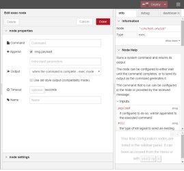
The Exec Node has one possible input and three possible outputs. For now, we’ll work with a
simple case in which we input anything into the Exec Node, which just runs the Exec Node unless
we specify, which we won’t specify. You type in your bash command in the ’Command’ section,
and make sure to have the ’+Append’ off for our case. The three outputs give three different
values, all pertaining to what running the command does to the Pi.
4.2 What We Did
Figure 10 shows a flow we created to run a python program and output it to our Node-RED
Dashboard site.
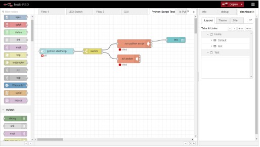
We start with a switch node that appears on the Dashboard site, which we won’t go in detail
about here. If you turn on the switch, it gives a boolean value True, which then goes through the
switch. The switch reads the value inputted and sends it to the specified path toward the ’run
python script’ Exec Node. The Exec Node sends the bash command “python test.py” to the Pi,
a test python program that outputs a short text every 3 seconds. It then sends the texts through
the top output of the Exec Node to the text Node, which outputs a text to the Dashboard site.
To kill the program, you flip the switch again on the Dashboard site, and it will send the boolean
value False, which goes through the switch and follows the path toward the ’kill switch’ Exec Node.
Here, it stops this specific program by sending the command “pkill -9 -f test.py”.
4.3 Is the Python Program Running?
We’ve been told by Evan that sometimes the Python programs have stopped running on their own
which is a problem. Here, we created a Flow that checks if a specific Python program is running.
Figure 11 demonstrates a Flow that’s sole purpose is to tell us if a specific Python program is
running or not.
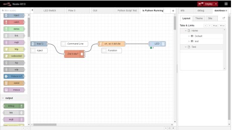
Ignore the white Nodes, they are just comments. It begins within an inject Node that repeatedly
injects a boolean value True every second. This runs the Exec Node with the command “pgrep
-fla test.py”. The outputs in the top output of the Exec Node always sends similar messages. In
fact, the text that is sent is indistinguishable until the 19th character. So, in the ’oh, so it did die’
Node it checks the 19th character to see if the program is running or not. It sends an On or Off
message to the LED, similar to the basic example from earlier. If the light remains on the program
is running, if the program has stopped for whatever reason, the light is off.
5 Plotting – NRPS
Plotting with Node-RED is generally straightforward, but very limiting given the skills and tools
we had while making these Flows and Nodes. Here will be a brief overview of what we’ve done as
a group.
5.1 Preliminary Actions – NR
Before beginning to plot, install a package titled ’node-red-contrib-graphs’. This package allows
for specific syntax when wanting to plot. To install a package, you go to the top right menu tab,
which looks like 3 parallel, horizontal lines, then go to ’manage palette’ and click on the ’Install’
tab and then type in the package you wish to install. You can also instead install it in the terminal
of whatever device you have Node-RED installed on by typing in “npm install node-red-contribgraphs” into the terminal. This is much quicker than the first option.
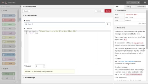
5.2 Live Plotting – NRPS
To plot live data is not too difficult. A not very extensive flow was created as seen on Figure 12.
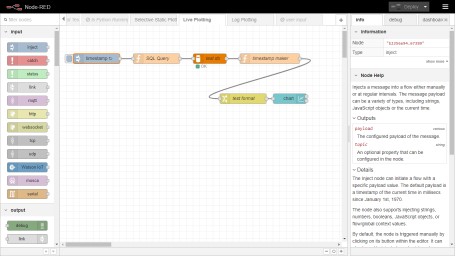
To allow for this to have a ’live’ feature, we utilized an inject node that injects at the same rate
that data is taken into MySQL, which is every 3 seconds in this case. Also, what is being injected
doesn’t matter, so we chose the standard ’timestamp’. The next Node is a function node that we
showed before, it sends a simple Query to MySQL, in this case the Query is:
Select*from rnts order BY id desc limit 50;
Where we plot the last 50 rows in our table. The next node is the MySQL node configured
to the appropriate database and table. After the MySQL node, where the data is pushed though
a msg object, is a function node that modifies the time stamp to match Node-RED’s dashboard
time preferences. It is in Javascipt, as most of Node-RED is. Here, the script goes as follows:
1 // loop through every row of the selected table
2 for (var i =0; i < msg . payload . length ; i++) {
3
4 year = msg. payload [i]. year ;
5 month = msg . payload [i]. month ;
6 day = msg . payload [i]. day ;
7 hour = msg. payload [i]. hour ;
8 minute = msg . payload [i]. minute ;
9 second = msg . payload [i]. second ;
10
11 // set up a timestamp object that is in the correct Node – RED Dashboard format (“
yyyy -mm -dd “+T+” HH:MM:SS “)
12 msg . payload [i]. timestamp = “”;
13 msg . payload [i]. timestamp = msg . payload [i]. timestamp . concat ( year +”-“+ month +”-“+
day +”T”+ hour +”:”+ minute +”:”+ second );
14 }
15 return msg ;
Succeeding that is a Change Node, that formats the data passing through to a format that is
legible for the Chart node. It is written in JSONata, which is a branch of JavaScript Object
Notation(JSON). First, you select a Change Node and alter some of the features. Figure 13 shows
us a Change Node that we modified.
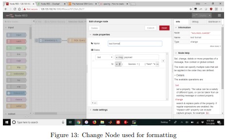
Under ’msg.payload’ there is an option to choose what’d you prefer to send. Click on the
button, which in default will show an “az” symbol which represents string format. Change the
selection to “expression”. Then, you click on the three dots to the right to modify the text. In
“expression” mode, it is by default in JSONata. Here is the code that is utilized in this expression.
1 (
2 $series := [
3 { ” field “: ” temp1 “, ” label “: ” Temperature 1″ },
4 { ” field “: ” temp2 “, ” label “: ” Temperature 2″ }
5 ];
6 $xaxis := ” timestamp “;
7 [
8 {
9 ” series “: $series .label ,
10 ” data “: $series .[
11 (
12 $yaxis := $. field ;
13 $$. payload .{
14 “x”: $lookup ($, $xaxis ) ,
15 “y”: $lookup ($, $yaxis )
16 }
17 )
18 ]
19 }
20 ]
21 )
All this does is parse through the y-axis data given, which are the two temperature values from
the example MySQL table from before. The x-axis is our timestamp, which we gave the specific
format for the Chart Node to read. In general, this code just prepares the data to be legible by the
Chart Node. To have more lines on the plot, hardcoding is needed since in this node we cannot
utilize loops or functions due to JSONata or possibly due to how unfamiliar we are with JSONata.
5.3 Chart Node – NRPS
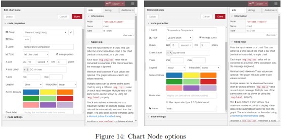
In Figure 14, the Chart Node’s set up is seen. First, the ’Group’ option is seen. Here, you decide
in which Dashboard subsection you’d prefer for your chart to appear on. Dashboard is a separate
website in which the Node-RED developer can show plots, bar graphs, virtual gauges, etc. To be
able to visually access the Dashboard, you simply go to:
{IP Address of device with Node-RED}:1880/ui/#/0
The ’Size’ option is somewhat limiting. The best way to find out what size you’d prefer is by
modify the sizes, then deploying, and see how it looks on the Dashboard. The ’Label’ option will
be the title of the plot. There are also different types of charts you can display, which is under the
’Type’ option. Most other options are self-explanatory, but the one to specify is ’X-axis Label’.
Here, you can set up in what units your time appears to be on the x-axis. It is written in a date
formatting string if you choose to customize it. Examples for a date formatting string can be found
here. You can also adjust the colors of the lines in your plot as can be seen along with choose
whether you want a legend to appear or not. There are many options to modify how your plot
looks, but it also seems more limiting than matplotlib. There are more customizable options with
plotting with the Template Node because you build a Dashboard tool from scratch, but we are
not fluent in html, JS, and CSS, so we had difficulty trying to navigate a program to plot on the
Dashboard with said Template Node.
5.4 Limitations – NRPS
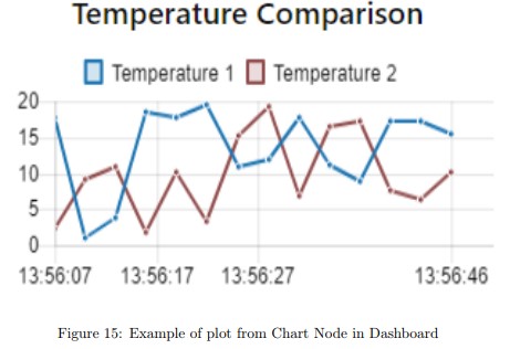
The Chart Node does not allow for axis to be labeled, you can substitute this with describing the
axis with the title. However, since the x-axis is exclusively time in the Chart Node and that it
does give you the option to format the time in any way you like, we feel that this is not too harsh
of a compromise to make. The legend at the top of Figure 15 is what appears when you toggle the
’Legend’ option on the Chart Node settings. We’ve been asked if we were able to plot any trace
given a selection but that now seems impossible with how the Node-RED Flow is built. We cannot
control the thickness of the plotted lines, which was also requested. We also do not know of a way
to add a data of when the plot was created. We have looked into alternative ways to set up our
Flows to allow for these options, but in general it seemed prone to bugs and would slow down the
quickness of the Flows.
5.5 Single Line Plot -NRPS
Now, as much as this sounds a bit backwards, it is much more straightforward to plot multiple
lines compared to just a single line. Even with following instructions left by IBM, the creators
of Node-RED, it would not plot a single line and nothing could tell us why. Instead there’s a
small work around. You should have a MySQL table that has the appropriate columns (id, data,
year, month, day, hour, minute, second, numTimeStamp). Everything in the flow is the same to
whatever kind of plot you want (live, static, etc.). Let’s look at the ’test format’ Change Node
from before. Originally we had this as the script for multiple lines:
1 (
2 $series := [
3 { ” field “: ” temp1 “, ” label “: ” Temperature 1″ },
4 { ” field “: ” temp2 “, ” label “: ” Temperature 2″ }
5 ];
6 $xaxis := ” timestamp “;
7 [
8 {
9 ” series “: $series .label ,
10 ” data “: $series .[
11 (
12 $yaxis := $. field ;
13 $$. payload .{
14 “x”: $lookup ($, $xaxis ) ,
15 “y”: $lookup ($, $yaxis )
16 }
17 )
18 ]
19 }
20 ]
21 )
Here we see the two fields of data, ’temp1’ and ’temp2’. Instead, we’ll leave the second one as an
empty variable of sorts. We’ll represent the field for the single data series as ’singleData’ and the
label as ’singleData Label’. Below is the script:
1 (
2 $series := [
3 { ” field “: ” singleData “, ” label “: “{ singleData Label }” } ,
4 { ” field “: “”, ” label “: “” }
5 ];
6 $xaxis := ” timestamp “;
7 [
8 {
9 ” series “: $series .label ,
10 ” data “: $series .[
11 (
12 $yaxis := $. field ;
13 $$. payload .{
14 “x”: $lookup ($, $xaxis ) ,
15 “y”: $lookup ($, $yaxis )
16 }
17 )
18 ]
19 }
20 ]
21 )
This plots the first data series, but nothing for the second field since it is empty. The only issue will
be you have a Legend set to ’Show’ on the Chart Node which will show two series in the Legend
labeled as ’singleData Label’ and an empty string. We recommend that when plotting a single line
to switch the Chart Node Legend option to ’None’ in this specific flow.
5.6 Log Plotting – NRPS
Log plotting is nearly identical to standard plotting. An extra function node is added in which the
y-axis data is sent through a logarithmic function.
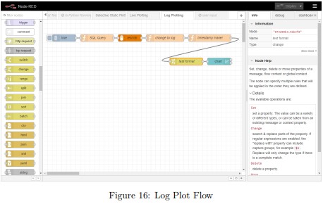
In Figure 16 the one added node can be seen. Nothing else in this flow has been modified
compared to the previous live plotting example. The ’change to log’ Function Node has the
following script:
1 for (var i =0; i<msg . payload . length ; i ++) {
2 var value = msg . payload [i]. temp1 ;
3 msg . payload [i]. logValue1 = Math . log( value );
4 }
5 for (var i =0; i<msg . payload . length ; i ++) {
6 var value = msg . payload [i]. temp2 ;
7 msg . payload [i]. logValue2 = Math . log( value );
8 }
9
10 return msg ;
Here, we just replace every value with it’s logarithmic counterpart and create a new object. To
have less or more lines to be log plotted, hardcoding this node is necessary, along with hardcoding
the ’test format’ Change Node.
5.7 Static Plot of Past Data – NRPS
Again, this plot does not vary much from the original live plotting example. However, this one has
one special attribute. Instead of having the inject node to begin the Flow, a Form Node is present
as seen on Figure 17. Here, user input from the Dashboard can be accessed.
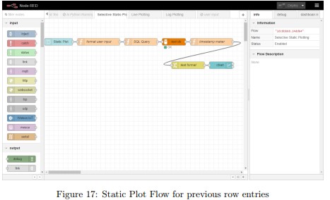
There is also a Function Node, following the Format Node, that modifies the user input to be
inserted into the query. Figure 18 shows the Form Node.
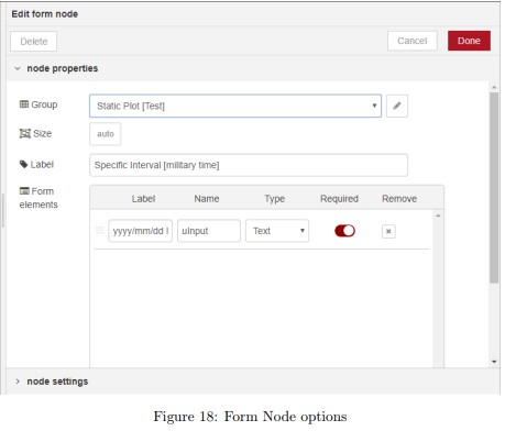
The form will appear in a separate tab in the Dashboard, which should match this flow’s Chart
Node’s Dashboard tab destination. Be certain both are destined for the same tab for ease of work.
The ’Label’ portion will be title of the Node and the prompt that appears to on the form in the
Dashboard. We specified how we wanted the user input to be under the ’Label’ column in the
’Form elements’ section. We specified users to use this format:
yyyy/mm/dd HH:MM:SS-yyyy/mm/dd HH:MM:SS
We then look at the ’name’ column which is important to remember. This name we used, ’uInput’,
will be the name of the object where the data of the user’s input will be stored. You can also
choose to have more than one form input, one being the first date and the other being the second
date, both with separate object names. You would need to be specific with objects and how the
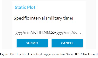
data is parsed in the following Nodes, which is not very difficult to implement. However, this Flow
uses the ’first timestamp – second timestamp’ notation. When deployed, this form will appear on
the Dashboard like Figure 19 shows.
This then feeds into a Function Node titled ’format user input’. The script for said function
node is below:
1 var str = msg . payload . uInput ;
2 str = str . replace (/:/g,””);
3 str = str . replace (/\ //g ,””) ;
4 str = str . replace (/ /g,””);
5 str = str . split (“-“) ;
6
7 msg . payload . date = str ;
8 return msg ;
Here, all all instances of ’:’, ’\’, and ’ ’ will be deleted, leaving two numeric time stamps similar to
the one seen on Section 3.2. These two numeric time stamps are separated by a ’-’, which we then
use the JavaScript .split() function that creates an array of strings based on the original string
that is separated by a specified character, which is ’-’ in this case. This array is set to an object
named ’date’ within the payload object. This object is then put into the Function Node that is
sends query commands to MySQL, as shown in Figure 13. The script for said Function Node goes
as follows:
1 msg . topic = ‘Select * from rnts where numTimeStamp > ${ msg . payload . date [0]} AND
numTimeStamp < ${ msg . payload . date [1]} ‘;
2 return msg ;
Here the query command specifies the interval of time based on the input given by the user which is
represented by msg.payload.data array. After this Node, everything is identical to the live plotting
example.
6 Acknowledgements
We would like to thank Dr. Henry Frisch and everyone in the PSEC group, in which there are too
many members to name. We would also like to thank the NSF for the grants in this REU and to
everyone who assisted in the organization and coordination in the REU. All of this allowed us to
gain more programming experience with multiple languages and to see how the application of the
Internet of Things can be successfully utilized in a laboratory setting.
Appendix A Installation
A.1 Pi Set-Up
The initial step is to set up a Raspberry Pi to be capable of the processing needs of Node.Red.
The password for the raspberry Pi currently being used in the PSEC office is “thegoodbook&”.
1. Enter apt-get upgrade into the command line because it is a package manager that will be
useful later on.
2. Enter the bash line “sudo raspi-config”.
3. Enter the root folder by entering “ïnto the command line.
4. Enter “sudo apt-get build-essential-essentials”, gets python integrated onto the Pi.
5. Enter “PIP” into the command line, is a Python integrated package
6. Enter” sudo apt-get install python-pip python-dev build-essential”
7. Enter “sudo pip install –upgrade pi”
8. Enter “sudo pp install –upgrade pi”
9. Enter “pip install numpy” for additional scientific tools onto the PI
A.2 Uploading Node.Red onto the Pi
To install Node.Red onto the Pi, use https://nodered.org/docs/hardware/raspberrypi , and follow
the criteria listed there, exempting parts of the document such as the rpi-gpio nodes, non-pi nodes,
and accessing the GPIO nodes.
To run node.red in terminal, use the command line “node-red-start”, with the server @http://127.0.0.1:1880/
The IP address is 128.135.102.16
A.3 Keyboard Configuration
Another important piece to the set up of the Pi an Node.red is proper keyboard configuration.
Raspberry Pi’s are typically set up with a keyboard of English gb, so it is important to shift over
to the American board.
To do so
1. sudo vi /etc/default/keyboard. This will take you to the configuration file where there will
be a piece with “gb”.
2. Press “i” to allow to insert
3. Change “gb” to “us”
4. Then press “esc” and “:x” to save
5. Enter command line “sudo reboot”.
The usefulness of this is that it will allow for proper use of “˜” in command lines.
Appendix B MQTT – Brokers and Clients
B.1 What is MQTT?
One purpose of Node Red is to be able to connect different devices without having to wire them
up. We want to be able to send a wireless message from, say, one computer to the Raspberry Pi.
This may be done in Node Red through MQTT, which is just a means of sending information.
B.2 Brokers and Clients
A broker filters messages and decides who to send them out to (clients). Take our example of a
computer trying to send a message to a Respberry Pi. How does the computer know where to send
the message? There can be millions of Raspberry Pis! We connect the Raspberry Pi and computer
through a broker. We can loosely think of the computer sending a message to a particular broker,
and the broker sending out that message to all clients subscribed to it. So the broker really acts
like the mailman delivering messages from on machine to another.
B.3 Downloading a Broker
We are using a free cloud-based broker, Shiftr.io.
1. Visit https://shiftr.io/
2. Sign up for an account. When creating an account, enter any profile name, enter your email,
and create a password. You will be asked to verify your email.
3. Once you are logged in, create a new namespace. A namespace is really just a folder for your
project.
4. After clicking “create namespace”, you will be redirected to your new namespace. Click on
“Namespace Settings”
5. Click “Add Token”. A token is basically a broker. You will be given a username (token) and
password automatically. Click “Create Token” to make the broker.
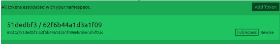
6. You will be redirected to a page where you will be able to see your created token. In my
case, the host server id is mqtt://51dedbf3:[email protected] . You will use
this in order to connect nodes and clients through the broker.
B.4 Connecting Nodes to Brokers
When connecting nodes together, it is important to establish a connection between brokers to send
information between nodes that are not connected through a direct connection.
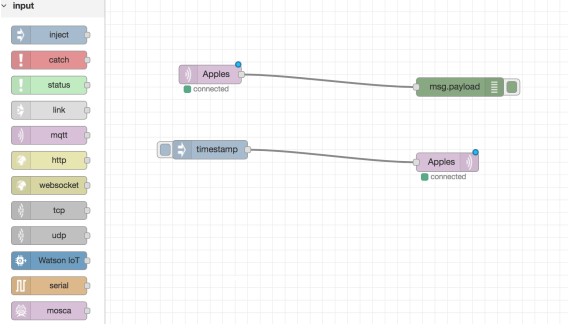
1. Input an inject from the input section, in order to then receive the message of a timestamp
that is transported from node to node using a broker.
2. Insert any number of mqtt, which is a messaging protocol. The example above is just an
illustration of what can be done. Be sure to also connect one debug from the input onto one
of the mqtt nodes in order for messages to be outputted.
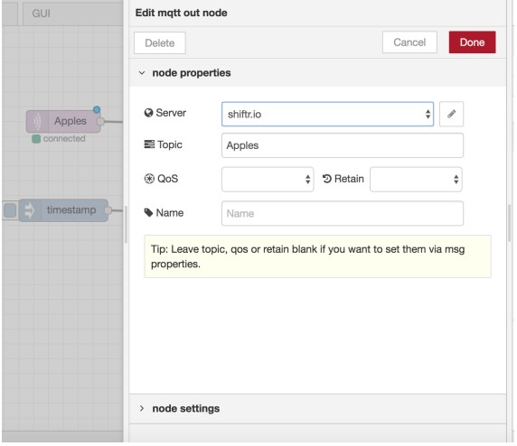
To reach the display page above, double click on one of the mqtt nodes. What is extremely important for creating a connection through a broker is for both mqtt nodes to have the same topic
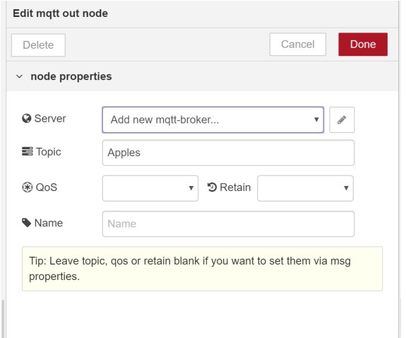
name (in this case, we use the word Apples). We must now connect the node to the broker. In the
server field, select Add New mqtt-broker… then click the pencil icon.
Then in the name field, enter Shif tr.io (really this can be any name you please). In the server
field, copy and past the host server id (this is from step 6 in section 4.3). Then click add and you
are all set. Do this for both nodes.
B.5 Downloading a Client
We are using a free client named MQTTBox.
1. Visit http://workswithweb.com/mqttbox.html to download.
2. Once the download is complete, open the app and click on “Create MQTT Client”.
3. Then in the MQTT Client name field, enter whatever name you would like. In the host field,
there may be some text already in entered, so delete in. Then copy and paste the host server
id from shiftr.io . In my case, it is mqtt : //51dedbf3 : [email protected] tr.io
which was mentioned in step 6 of section 4.3. But we must make some alterations. Erase
the mqtt : // component of the host server id (it turns out, MQTTBox automatically enters
this piece for you when you create the client, so you should not put it in yourself.). Then
at the end of the server id, add :1883 (yes including the colon). The number you just added
is called the port number, which identifies the port at which the broker may be found. It
will always be 1883 in our case. The entry in the host field should look like this in the end
51dedbf3 : [email protected] tr.io : 1883
In the protocol field, select mqtt/tcp. Click save
4. After saving, you have created a client!
You can use a client to send messages to nodes (and other clients) subscribed to the same
topic (subscribe just means they have the same topic, so they get messages about anything
else with that topic).
5. Now let’s send a message to our nodes in node red which we set up in section 4.4. In our
client, add the same topic as before (in our case Apples). Then type in Hello in the payload
field. Click publish
6. Return to the the node red program flow from earlier. Click on the debug tab on the top
right of the screen. You should see the message.
Acknowledgements
I would like to acknowledge Roy Garcia who contributed to setting up the MQTT Broker and
MQTT Client. He also contributed to creating the dashboard display for the plots.
Source: Node-RED.