
IMAGE PROCESSING DETAILS
The OTS MGS evolved across three main iterations. The driving system requirement of these iterations was processing all image analysis and feedback within 100ms per frame, or 10fps.
First Iteration:
Image processing starts with the loading of a video frame into memory as an image file. The microcontroller then iterated through the individual pixels of the image while applying a “connected component analysis†algorithm to identify a pixel of the appropriate laser color (e.g. Red > 200). This was all done in the RGB color space. The algorithm will then examine its neighboring pixels for the same color, expanding this procedure until all same color pixels are identified. This is a recursive call that will add each red pixel to a set. This set, now containing the pixels representing the image of the laser, can be analyzed to identify the center of the image, and thus the POA indicated by the laser. Identification is performed by averaging the minimum and maximum x and y pixel values in the pixel set. The laser beam will be a reasonable approximation of a circle, allowing this method to determine the center point of the laser image with reasonable accuracy.
Results of First Iteration:
This method proved to be much slower than our stated requirement, taking an average of 1.5 seconds per frame, or 0.66fps. It was determined that loading each frame into memory as an image file, in this case a jpeg format, was consuming a significant amount of the processing time. It was also found that accessing the individual data for each pixel was creating further delay.
Second Iteration.
Connected-Component Analysis was ruled out and a different method was sought. This resulted in a second iteration derived from open-source code available from the OpenCV community. This code acquired an image but stored it as an array, not converting it to an image file. It then converted the image array into the HSV (hue, saturation, value) color space. The HSV color space is better because it is easier for the human eye to discern colors in than the RGB color space (which is better for computers). After converting to HSV, we used the inRange function to filter the colors for the laser light. Adjusting the range of values used in thefilter was implemented using on-screen trackbars to allow the user to tune the system for their lighting environment. What results is a white value for pixels within our range, and black for those outside our range. We then applied erode and dilate transforms which smoothed out the image. These transforms are part of the OpenCV library, an open source computer vision library. This code then identified circles using a HoughCircle function. This function is a variation on the Hough Transform, an image extraction algorithm, that identifies circles within a range of radiuses.
Results of Second Iteration:
This was much faster, but it would often identify many circles and it was very difficult to filter which of the circles was the laser. There were often many false positives that would skew our results. Also when the laser was smaller than 7-8 pixels wide it could not be found.
Third (and final) iteration:
The third and final iteration was still done with OpenCV libraries, but uses contour identification to find the circle. The same filtering process is done with conversion to HSV space, then filtered for a range of colors. No image transformations are applied. After being filtered it is sent to the findContours function, which identifies the contours in the image sort of like a topographic map. What is returned is a hierarchy array which has the data for each of the contours. When contours are found, it is easy to iterate through the hierarchy of contours, establish a moment on them, and find the area and centroid (center x, y) of the shape. We then filter for a minimum/maximum area of our laser pointer.
Results:
This was not only the most accurate iteration, but also the fastest, running at more than 30fps.
HAPTIC FEEDBACK DETAILS
In order to make the motors apply different levels of vibration, the motors must receive different DC values. Since there is no analog output on the pi, the simple workaround is using PWM (pulse width modulation). By varying the duty cycle on this output signal, essentially a different DC output is created.
Programming PWM
Our feedback on the pi uses a library called pigpio. It is written in C, but has a very simple and function python client that it runs on. In order to use it, the daemon must first be started via command ‘$ sudo pigpiod'. This daemon allows the program to continue servicing the PWM output in the background. Pigpio allows the program to choose any of the GPIO pins and set the frequency and duty cycle at any time.
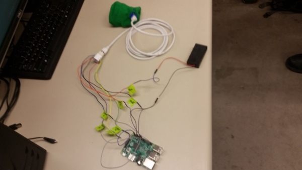
Figure 1: Assembled Raspberry Pi and Haptic Feedback System
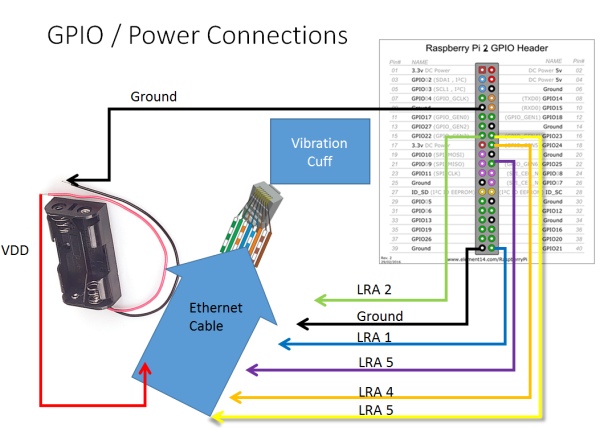
Figure 2: Raspberry Pi Header Wiring Diagram
VIBRATION CUFF
The vibration cuff is composed of a flexible plastic backing with five Linear Resonant Actuators (LRA) controlled by TIP31A NPN BJTs. All of these transistors are connected to a CAT5 Ethernet port, allowing a simple patch cable to act as a parallel cable, utilizing seven of the eight connections. The 28 AWG wires that compose the CAT5 cable are capable of handling 577 mA current, safely above the 400 mA worst case current draw found in Chapter 4. This incorporates a near universally available connector and data cable that can be readily sourced or replaced if damaged during use. From the GPIO pins on the Pi, Pulse Width Modulation (PWM) is then used to scale the voltage across the transistor bases and control the current to the LRAs. This assembly is then fit into a soft wristband to be worn by a user. The choice of LRAs over the competing ERMs was made after discovering the extreme heat and current draw of the ERMS. The ERMs drew a peak current of 520 mA at 4V, and produced noticeable heat when tested. They were further disqualified when the protective housing created for them failed to prevent seizure of the rotating mass and subsequent motor stall. In comparison, the moving mechanisms of the LRA motors are fully encapsulated in a hard plastic casing and draw at worst 80 mA of current at 3.3V, or 15.3% of the ERMs. The LRAs were a better choice because they are safer and use much less power.
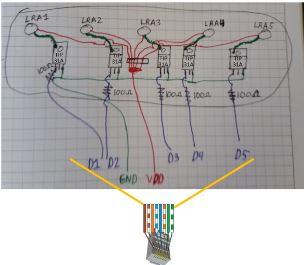
Figure 3: Wiring Diagram for Vibration Cuff
VALIDATION OF DESIGN
As it is shown in the figure, the vibration system consists of five LRA vibration motors, five TIP31A transistors, five 100 ohm resistors and several wires. Each LRA vibration motor has similar but different characteristics. During the testing of those motors, Agilent E3611A DC Power supply and HP 34401A Multimeter are used to precisely measure the voltages and currents in each iteration. The Agilent E3611A 30W single-output power supply features separate digital-panel meters for monitoring voltage and current simultaneously, giving precise reading and control capability. The E3611A features 10-turn potentiometers for accurate adjustment of voltage and current output settings. Also, the 34401A provides a combination of resolution, accuracy and speed that rivals DMMs costing many times more, 61/2 digits of resolution, 0.0015% basic 24-hr dcV accuracy and 1,000 readings/s direct to GPIB assure you of results that are accurate, fast, and repeatable.
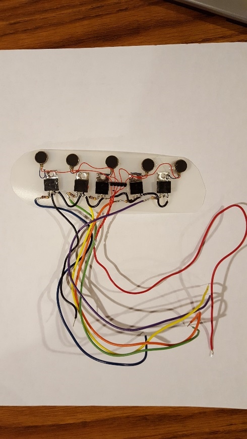
Figure 4: Completed Vibration Cuff
To measure this data, two banana connectors were used to connect the power supply and multi-meter first. Then using the grabber wires to catch the positive and negative pole of each vibration motor respectively. The next step is measuring the values of both voltages and currents displayed on the power supply with rotating the knob of voltage. It is apparent that all five motors work well. The reason why the measurement stop at 3.3 volt is because 3.3 volt is the maximum output limit for the Raspberry Pi. The currents slightly increase when the voltages jump from 0 to 3.3 volt.
Our tests showed that the minimum activation voltage was 600 mV with a current draw 10 mA. The LRAs demonstrated sensitivity up until 1 V, where an increase in vibration was no longer discernable and current rose quickly. At the 3.3V maximum Pi output GPIO voltage, the peak current draw was measured at 80 mA for LRA4. Using this as a worst case scenario motor, the total maximum current draw would be 400 mA for all five motors.
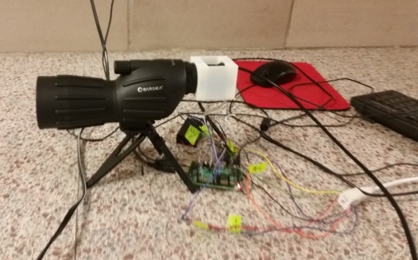
FINAL PROJECT
Below is an image of the camera connected to the spotting scope, fully set up with the Pi.
Source: Precision Pointing Device