Underwater 3D Data Collection

1.0   Introduction:

How can you call this planet earth, when it is quite clearly water?

On average, 1,582 shipping containers of cargo have been lost at sea each year over the past nine years (World Shipping Council, 2017). These lost containers, however, only make-up a fraction of marine anthropogenic litter. A rough estimate by the United Nations Educational, Scientific, and Cultural Organization claims that there are more than three million shipwrecks at the bottom of the ocean which remain undiscovered to this day (UNESCO, 2007). Furthermore, within some of these wreckages is an estimated $60 billion worth of lost treasures and relics (Sean Fisher, Mel Fisher’s Treasures, 2012). Despite this, lost fishing gear makes up the largest portion of plastic pollution in the world’s oceans. It is estimated that over 64,000 tons of abandoned nets, fishing lines, and traps are deserted in the ocean. A recent study examined a sample of 42,000 tons of plastic waste found in the ocean, 86 percent of which was made up of lost fishing gear (Laville, 2019).

While any lost items on Earth’s mainland may be easily recoverable, the same cannot be said for what lies at the bottom of the sea. More than 80 percent of the ocean remains unmapped, unobserved, and unexplored (NOAA, 2018).

In order to combat this lossage, various recovery initiatives have been started. These programs range from ocean clean-ups to utilizing technology to obtain a more detailed image of the ocean floor, in turn leading to a greater ability to identify where lost items are located. In January of 2019, environmentalists collected 40 tons of abandoned fishing nets from the Pacific Ocean over the course of 25 days (AP, 2019).

According to the National Oceanic and Atmospheric Administration (NOAA, 2018), only 35 percent of the United States’ coastal ocean waters have been scanned and mapped with modern methods. Since the utilization of underwater vehicles to research the ocean is an expensive practice, other forms of technology are used to visualize the ocean floor in a more efficient way. Sonar is the most common technology used, however less than ten percent of the ocean floor has

been mapped with technologically adequate sonar devices (NOAA, 2018). Many up-and-coming companies are joining the push to use sonar to produce a better image of the ocean floor, as well as to locate lost items. In 2017, one such company, Ocean Infinity, created a collection of eight underwater drones packed with sonars that has the capability to cover five times more area than sonar devices from a decade ago. This company, working in conjunction with another startup, plans to have the entire ocean floor mapped by 2030 as part of an initiative called Seabed 2030. Within the past two years, this program has helped increase the percentage of the ocean floor mapped from six percent to fifteen percent (Wise, 2019).

This information proves that a modern solution is the best choice in order to better locate lost marine litter in an efficient and effective manner. Over the past few years multiple technologies capable of accurate 3D data collection have been created or optimized to ultimately produce better results ultimately satisfying this data collection requirement.

1.1   3D Data Collection and Object Detection:

Such examples of technologies capable of detecting and producing an image of underwater objects are radar, lidar, and sonar, however, some are more capable than others. Each technology depends on the fundamentals of an echo to detect an object within its environment. Essentially, a wave is transmitted into open space and the time elapsed for each wave reflection that travels back to the origin is measured. Radar uses radio waves to do this, while lidar uses light waves, and sonar uses sound waves. There are trade-offs for using each detecting technology which depend greatly upon the physical constraints of the surrounding environment.

1.1.1 Radar:

Radar has been in use since the late 1800s century when it was used by Heinrich Hertz in his experiments which determined that radio waves can be reflected by metal objects. It was not until the 1900s when radar was put to practical use by Christian Hulsmeyer who created a ship detection system allowing for ships to navigate in foggy conditions. It was in the 1930s when radar became popular among other European countries and the United States, as radars were being further developed by militaries for aircraft detection in World War II (Kostenko, 2003).

The actual term, RADAR, was created by the United States Navy in 1940 as an acronym for Radio Detection And Ranging (Translation Bureau, 2013).

Radar is a common detection system composed of two major pieces which are used to determine the distance, location, and speed of objects. It uses the transmission of radio waves to detect such objects. The radar system uses a transmitter to produce electromagnetic waves in the radio and microwave frequency range. A receiver then is able to detect any waves that have been reflected back from the target object which then allows the user to determine the properties noted above based on the time, speed, and angle of the return waves (Olsen, 2007).

The first radar applications were used in the military as they allowed locating targets on the ground, in the air, or out at sea. As radar technology developed and became more widespread, it began to have civilian applications as well. Today commercial airplanes use radar systems to help them land in poor visibility conditions. The Air Force still uses radar systems on their planes to assist in detecting and tracking enemy objects. Radars are used in a similar way for marinecraft. They can be used at sea to determine the location of islands, buoys, and other ships allowing one to orient themselves on the water. One very common application of radar that does not involve the tracking of other vehicles is weather radar. Meteorologists use radar to detect and track precipitation for short term weather predictions (Olsen, 2007).

There are several advantages to using a radar system over other detection methods. As mentioned above, radar is useful in detecting objects that may not be visible due to weather conditions. Radar can penetrate clouds, rain, fog, and snow. Additionally, radar is able to penetrate insulating materials like rubber and plastic due to the frequency of the radio waves that are used. Other benefits of a radar system includes its ability to measure the distance of a target, ability to locate the object, and ability to collect information quickly. It also allows for 3D images to be created based on various angles of the return signal in relation to the target object (Pen-Jui et al., 2015).

Radar does have its drawbacks as well. Radar’s transmitted signals can be interfered with by several objects and mediums during the time of flight of radio waves (Olsen, 2007). Additionally

it is unable to detect objects that are too deep in water, nor can it detect the color of an object. Finally it does not perform as well as other detecting systems in the short range (Payne, 2010).

1.1.2 Lidar:

The first laser was invented in 1957. Shortly after this discovery, in the 1960s, the concept of utilizing lasers to measure objects was first used by the National Center for Atmospheric Research. Lasers were used in combination with radar to measure the size of clouds (Bornman, 2015). Light Detection and Ranging (Lidar) then began to increase in public popularity after it was used in the Apollo 15 mission to generate maps of the moon’s surface. Following this, the National Aeronautics and Space Administration (NASA), among other organizations, used lidar throughout the 1970’s for various tasks, most commonly topographic mapping (Gaurav, 2017). By the 1990’s lidar scanning technology had begun to be rapidly developed and improved due to its potential for high resolution data outputs. Lidar technology continues to be improved today, most notably in the accuracy of the data generated and the amount of points generated by the scanners. Currently, NASA is working with the U.S. Geological Survey (USGS) on a project called the 3D Elevation Program, to create a nation-wide lidar dataset that includes the topography of the United States (USGS, 2017).

Generally speaking, lidar is a surveying method that precisely measures a distance to a target using laser beams of light. Initially, a sensor sends pulsating lasers in the direction of a target to be measured or modelled. Once the laser returns to the receiving part of the sensor, the time elapsed between the emission and receipt of the laser beam is recorded. This time measurement is known as time of flight (Hu, You, & Neumann, 2003). The scanners have the ability to generate thousands of measurements per second. These measurements are then pieced together to create a point cloud of x,y,z coordinates of the object or surface being scanned (Pfeifle, 2012).

Historically, lidar has been commonly used in applications revolving around urban planning, mapping topology, and tracking geological changes over time (Inomata, Triadan, Flory, Burham, Ranchos, 2018). Due to the generation of complex and accurate datasets generated by lidar, accurate models in these areas are able to be studied and edited to reflect the needs of the user.

Recently, lidar has been used increasingly in conjunction with the development of autonomous

vehicles. Lidar’s ability to locate potentially hazardous objects within a vehicle’s path of motion allows the vehicle to calculate the best way to avoid collision (Velodyne Lidar, 2018).

The high accuracy of data generated by lidar scanners remains one of its largest advantages. Additionally, the large amount of points created by the pulsating lasers creates a high sample density allowing for extremely accurate models. However, lidar scanners can be very expensive. The high sample density also requires a high level of processing in some applications before it can be used as required (Lidarradar, 2018). Since lidar relies on the visible spectrum to retrieve and generate data, it becomes more complicated to use underwater as the speed of light slows.

Therefore, when the data is captured underwater, it is more susceptible to noise and the high level of accuracy normally expected from lidar can be negatively impacted.

1.1.3 Sonar:

Although bats have been using this method of location for generations, it was 1916 by the time people figured out how to replicate this process. Paul Langevin created the first working model of a sonar. It was crude and took a large amount of power, but in only two years he and Constantin Chilowsky had refined the project to be able to detect metal from 200 meters away (Graff, 1981). Though active sonar would still require a lot more refinement before use, passive sonar was in use to find nearby submarines during World War I. The Germans were the first to publish a paper on the sonar effect, listing a number of its issues such as interference and short range, but this paper was ignored for a long time. During World War II, a simple but effective active sonar had been developed and was crucial in fighting German U-boats. After World War II, research and development on sonar slowed massively. Though advancements were made, nothing major has changed since World War II (D’Amico et al., 2009).

Sonar is the process of using soundwaves to locate objects. This is done by having a transmitter and receiver in one location. The transmitter emits a sound wave that propagates through the medium. When the sound wave hits a solid object, it reflects back to the source as is picked up by the receiver. This receiver informs the system that a signal has been received. The system, knowing the time difference between when the signal left and was received can then estimate

how far away the object is. Using multiple measurements determined from these sound waves, a picture can be created of simple objects (Waite, 2002).

One of the most common uses of sonar is for boats to detect underwater objects like submarines or fish. Since sound travels through liquids and solids with ease, it has proved ideal for locating objects in the water. Sonar is used to find a number of things such as fish, boats, plane crashes or mines, yet sonar can also be used to look through objects. Ultrasound is another use for sonar and is commonly used to look inside of living creatures.

The biggest strength of sonar is to see through solid or liquid mediums. It is a low-cost setup to be able to map and find objects hidden from view. Yet sonar is very susceptible to noise and dispersion. This makes it non-ideal or long-range detection. Lower frequencies can be used to increase the range, with a loss to resolution. Another issue is that sea wildlife is a major issue for sonar if it is transmitting at similar frequencies to wildlife (Payne, 2010).

2.0   Background:

In this section, the method of 3D data collection chosen to be used for this project is discussed. Additionally, previously done experiments using various sonar devices are analyzed in order to better understand sonar operation. From there, methods to maximize device efficiency are outlined and a summary of how this device will help in the solution to the problem of locating marine litter is detailed.

2.1   Chosen Method – Sonar:

Essentially, the overarching problem at hand is the large amount of objects that are lost at sea each year. Although shipping containers make up a large percentage of this marine litter, common items lost by anyone using the water body add to the total amount. Having a system in place to locate these lost items would help to recover them from the sea floor. Based on the initial problem at hand and the advantages and disadvantages of each data collection technology discussed above, it has been determined that sonar would be the most effective method to identify and visualize marine litter and debris.

However, various attributes of sonar scanning technologies have to be considered in order to derive the engineering requirements for the final solution. Each attribute has trade-offs that will affect the performance of the final system.

2.2   Understanding Sonar Functionality:

This section goes over the various forms of sonar and the advantages and disadvantages of those systems.

2.2.1 Types of Sonar:

Primarily, there are two types of sonar systems, passive and active. Passive sonar consists solely of a hydrophone, also known as a microphone. Active sonar devices are comprised of a projector, or transducer, in addition to a hydrophone (Waite, 2002).

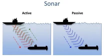
Passive sonar is used to receive sounds, or noise, generated within the water. This noise is generated by various sources including biological life and other vessels. Since only a hydrophone is used, no signal is emitted from passive sonar systems. Due to this, it is commonly used in military applications when underwater vessels do not want to emit their own noise (NOAA, 2018). Additionally, passive sonar does not give information about the range, or distance, of the target it is sensing. Instead, it generalizes that an object is in the vicinity of the sensor. However, if the passive sonar is used in combination with other passive sonars, the location of a target may be calculated through the use of triangulation (Waite, 2002). The equation to calculate the signal- to-noise ratio (SNR ) for passive sonar is given by SNR (decibels) = SL – TL – (NL – AG). In this equation, SL refers to the source level of the signal transmitted by the sonar. TL refers to the transmission loss, in decibels, which explains how much signal intensity is lost when detecting objects further away. TS is the target strength which also lessens the further an object is away from the sonar. Finally NL is the noise level in the water and AG is the array gain (Discovery of Sound in the Sea, 2002).

Active sonar generates a pulse of sound through the transducer. When a target is in the path of the pulsating soundwaves, the target reflects the waves. Finally, these waves are received by the hydrophone. In some cases, the strength of the return signal can be recorded as well. Similarly to lidar, the time of flight is calculated as the difference in time between the emitted signal and the received one. The combination of multiple pulses serves to detect the location of an object in the

water (Waite, 2002). The equation to calculate the signal-to-noise ratio (SNR) for active sonar is given by SNR (decibels) = SL – 2TL + TS – (NL – AG) (Discovery of Sound in the Sea, 2002).

Commonly, two types of active sonar are used to detect objects within, and to map the ocean floor. They are known as side-scan and multibeam sonar. Side-scan sonar is preferred for underwater object detection. Side-scan sonar consists of a device to send and receive sound waves, a transmission cable, and a data-processing computer. The computer records and plots received data points to assist in the visualization of the object. Side-scan sonar is usually orientated downwards towards the ocean floor. As it moves, the beams record the changes in the ocean floor (NOAA, 2013). Multibeam sonar consists of multiple transducers that allow the scanning of a larger area at once. The beams emitted from the sonar are in a fan shape (NOAA, 2009).

2.2.2 Sonar Targets:

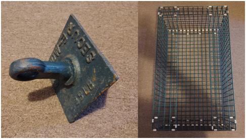
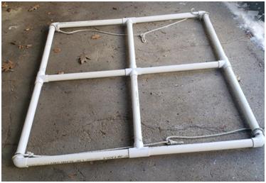
In order to accurately utilize the capabilities of sonar, multiple tests consisting of various targets moving at different speeds and locations relative to the sonar are required. Targets can consist of any physical structure placed in the field of view of the operating device. In this case, three targets were used to conduct testing a decommissioned lobster trap, a 25 pound anchor, and an enclosed cross built out of PVC piping.

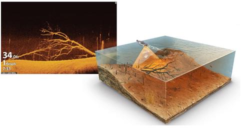
2.2.3 Side Imaging and Down Imaging Sonars:

In order to better understand the output data displayed from commercially available sonar devices, data from multiple tests was reviewed. The main purpose of this was primarily to understand the difference between down imaging and side imaging as it is viewed in a real world setting. Various recordings that had been previously collected were examined. These recordings depicted the above anchor target being maneuvered in different ways in front of the sonar devices doing the recording. A detailed list including the sonars used and the tests performed can be found below.

The first recording captured an anchor being lowered to the sea floor then raised back up. This recording was captured using down imaging through a Garmin 53CV chartplotter (Michalson 2019).

The next recording depicts the same anchor being lowered, while regularly being held at various intervals in the water column. This was repeated until the anchor neared the sea floor, then the same process was repeated on the way back up. Down imaging was used for this recording on a Garmin 53CV chartplotter as well.

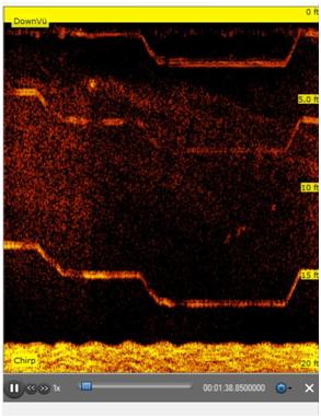
These tests capture the functionality of using down imaging in sonar devices. For each test, a path of motion is clearly defined and matches what was expected from the description of the test. As mentioned previously, down imaging captures objects below the sonar device by emitting sound pulses towards the object perpendicular to the water body floor. The above recordings confirm this, showing only a single view of the target in motion.

Next, a recording was examined to better understand the properties revolving around side imaging sonar devices. Once again, an anchor was lowered to the bottom of the sea floor and raised back up. This recording used the side imaging feature on a Garmin 73SV chartplotter.

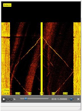
The anchor’s path of motion is again clearly visible in this recording. However, the primary difference between side imaging and down imaging is captured. As seen in the figure above, the transducer emits a wide range of pulses during side imaging that capture protruding objects on both sides of it, parallel to the water body floor. Because of this, the anchor’s motion can be seen on two sides of the recording, with the yellow line representing the transducers path.

An important aspect of using both side imaging and down imaging is that the resulting recordings track the motion of the target. Additionally, these two types of imaging depict targets solely in two dimensions. The combination of these features are responsible for the anchor’s path of motion in all tests being represented as a line, rather than a three dimensional image on an anchor.

2.2.4 Three Dimensional Imaging Sonars:

The recordings where the anchor was used as a target were intended to view how two dimensional sonars capture object motion. However, some applications require a three dimensional image of the target being located. In these applications, three dimensional imaging sonars are commonly used. In order to better understand the difference between these types of sonars, further recordings were observed using sonars capable of three dimensional imagery. For these recordings, the other two targets, a lobster trap and PVC cross were used. While the above recordings capture a moving target, the three dimensional sonar recordings were done using stationary targets. These recordings were made using a Sound Metrics Aris Explorer 3000 (Pulsone, 2019).

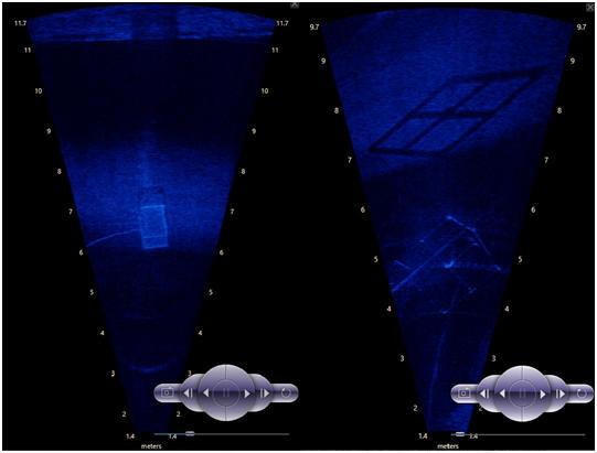
With this type of sonar, a better three dimensional image of the target as a whole is captured. The above image on the left indicates the lobster trap and the image on the right indicates the PVC cross. In both recordings, the three dimensional shape of the target is more clear than when using

side imaging and down imaging. Additionally, the measurements on the side represent the range of the sonar in whatever direction it is pointing, rather than only indicating the depth of the water body. When the targets move in the field of view of a three dimensional imaging sonar, the path of the object is not captured. Instead, the object is simply seen to be moving similarly to the way an object would move in a recording done using a video camera on land.

Overall, these recordings demonstrate some various types of common sonar devices on the market today. Understanding the difference in functionality and data output from these different devices is important when determining the best approach for original sonar design. Each type has various advantages and disadvantages, making application a significant factor when deciding which sonar to use.

2.2.5 Operating Environment:

When dealing with underwater data collection, a large variety of environments may be encountered. These may range from shallow and clear to deep and turbid aquatic areas. In addition, the operating environment can be a controlled area, such as an indoor swimming pool, or a natural water source such as a lake, river, or ocean. Each of these areas influence the way sonar data is collected and processed.

Typically, a maximum operating range for sonar devices is between 10 and 100 kilometers (Smith, 2003). However, due to the nature of this object detection project, only underwater distances up to a few hundred meters will be considered as the sonar will be collecting information of the waterbody floor directly below it. When working in various depth levels, sonar will perform better in shallower environments allowing for a clearer image to be produced. This is because the acoustic beams being reflected off marine floors closer to the transducer will be at greater intensities and more numerous as they are not being lost due reflections and unable to be received back at the source of the transmit. Additionally, a larger amount of beams sent to the object will return when the distance travelled is less, as the beams will come in contact with the object at a higher concentration (NOAA, 2013).

As mentioned previously, the clarity of the water source influences the quality of scanned data. Objects scanned in clearwater echo sound waves better than objects in dirty water as less beams are lost to floating particulates. Also, objects in darker water lose the ability to reflect strong beams, resulting in an object image with lower resolution (NOAA, 2013). This, however, is not a major potential issue as sound wavelengths are 2,000 times longer than light wavelengths, allowing for the waves to move around suspended particles in the water that would otherwise block and scatter light waves (Soundmetrics).

2.2.6 Data Collection Rate:

When collecting the underwater 3D data, it is important to consider the rate at which it is being collected, as this may affect the ability to properly identify any man-made structures submerged at the bottom of the body of water. A main factor is the speed, or lack thereof, at which the sensor is moving, as it will likely be attached to a marine vessel.

When collecting data with fish finders, which utilize sonar technology to locate fish or underwater structures, the boat speed influences the resolution of the observed image. A general rule of thumb is that the faster the boat is travelling, the less detailed the image will be.

This is because the sonar device will emit the same rate of sound waves in a certain time travelled, regardless of the speed. As a result, a faster speed will spread out the areas where sound waves are reflected back to the receiver, ultimately decreasing the quality of the image (Martens, 2017). Depth also influences the image resolution in relation to speed travelled. Faster speeds will not sacrifice image quality in shallower areas as less time is needed for the sound waves to hit the target and return to the sonar. Essentially, depending on the depth of the area being scanned, there is an ideal speed to move the sonar in order to receive an image of sufficient quality for the project being conducted (Martens, 2017).

2.2.7 Data Resolution:

The size of the beam being used during a scan will affect the amount of detail, or resolution of the picture that is obtained from objects and structures underwater. As mentioned previously, sonar works by emitting a pulse of sound waves to detect objects. As these waves travel through space they expand into cones becoming wider the further they travel. Many sonars give the user

the ability to control the scanning frequency which then ultimately affects how wide the sound wave cone will be. Using a wider beam is suitable for scanning a shallow area quickly. As the water becomes deeper the cone becomes wider. Eventually it will reach a point where the sound waves have become so spread out that no reflections will be received and objects at that depth will not be detected. Narrow beams are more suitable for detecting objects at greater depths since the cone will not spread as wide and reflections will be obtained. A lower frequency will result in a wider beam while higher frequencies will result in narrower beams (Deeper).

2.2.8 Data Visualization:

Common methods of sonar data visualization include side imaging and down imaging. Each method produces a different type of image that brings with it various advantages and disadvantages depending on the intended usage.

Side imaging sonar is most commonly used to view the bottom of a water body floor. It relies on emitting sound waves horizontally across the bottom of the water body. During this process, objects extruding from the floor will reflect the waves back to the sonar device. Based on the emission geometry of side-imaging sonar, it is commonly used to search for debris, such as shipwrecks (Enviroscan, 2020).

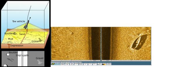
The images above display a diagram showing side-imaging sonar as well as an example of data visualized from a fish finder. As seen, the produced image displays the objects along the side of the sonar, parallel to the water body floor.

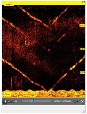
Down imaging sonar emits sound waves vertically from the bottom of the device. The returned image represents the structure of the floor below the sonar device and perpendicular to the sonar beams. Objects within the frame are also displayed. As the sonar travels along the water, whatever objects are immediately below it reflect the signal and are then displayed on the device (Humminbird, 2019).

The above photos display an example of down imaging data visualization as well as a diagram of sound wave emission from the sonar.

2.2.9 Power Consumption:

The sonar equation is used to estimate the signal to noise ratios (SNR) for sonar scanning systems. The SNR is ultimately what determines how well the receiver of a sonar system will be able to detect the reflection of a pinged signal through the background noise present in a body of water. The SNR takes into account the level of the signal’s source at the origin, the spreading effects of the signal through the water, the absorption of the signal through its environment, reflection losses, ambient noise, and the characteristics of the sonar’s receiver (Urick, 1983).

Through utilization of the sonar equation and the SNR, one is able to determine the required transmit power to account for all of the factors mentioned above that will affect the signal over time as it is transmitted, reflected off of the target, and received back at the source of the sonar. For a given total power output, the intensity will be reduced as a function of range as the same amount of total power (Federation of American Scientists, 1998).

2.2.10      Mechanical Attributes:

As with all systems, various mechanical considerations need to be made prior to attaching a sonar device to the object in motion. Common methods of sonar attachment are towing and mechanical fixturing. Towed sonars, commonly used for defense, are dragged behind an aquatic vessel. They are attached to the vessel by a wiring system often released off the back (ACTAS). Additionally, other sonar devices such as fish finders are mechanically fitted to the boats where they are used. This is usually done by means of screws or brackets provided with the fish finder. Then, the transducer is fitted underwater on the edge of the boat. When the device is mechanically attached, it is important to consider physical properties of the device that need to be counteracted. For example, the bracket or bolt set needs to be strong enough to prevent device breakage as a function of both water resistance during motion and the sonar weight.

Additionally, the transducer needs to be fitted to the boat strongly enough to counteract forces imposed on the device as it travels through the water. It is important that the transducer is fluidly dynamic to limit the effect of water resistance on the system.

2.2.11      Potential Hazards:

There are a number of hazards that are present while operating electronics nearby water. The water presents a notable risk to all the electronics enclosed in the sonar, meaning that the board will need to have watertight protection. These electronics also present a risk to nearby surrounding animals if the watertight protection were to fail.

There is also a hazard present if certain frequencies are used. Some frequencies are harmful to sea life and can lead to injury and even death. The first sonar system developed by the navy would generate 235 db, while the worlds loudest rock band only produced 130 db. These high decibels also present a notable risk as they can easily begin to cause damage (Scientific American, 2009). The Navy has also admitted that their experiments have caused over 3 million marine mammals to be injured and 2 million people to have temporary hearing loss (Naval Facilities Engineering Command, 2018).

2.3   Derived Engineering Requirements:

In this section the final engineering requirements for the system will be discussed followed by a general block diagram to help the reader visualize the final system. For each of the attributes of sonar described above, a general decision will be made determining which property to focus on during the construction of a new sonar device in order to solve the initial issue presented.

Due to the fact that passive sonar does not easily provide the distance or location of an object, a variation of active sonar will be used to detect marine litter and debris. Since active sonar has the ability to send pulses of sound and record the distance travelled until their return, it is better suited for the purposes of locating submerged objects.

Regarding the operating environment, a controlled and clear water body of varying depths, such as a swimming pool, will be used, allowing data to be collected efficiently. A controlled environment will allow focus on sonar concepts such as effective data visualization of targets of a known size and location without having to consider the large amounts of noise encountered in turbid aquatic systems. This way, conclusions can be made regarding the practice of locating objects and applying these conclusions to natural water bodies.

The data collection rate and data resolution will depend largely on the constructed sonar device discussed. Additionally, once sample data is collected and the average size of this data is analyzed, a decision will be made about the necessary amount of on board data storage available. Once these decisions are made, a display will be selected that can accurately show data of the intended resolution.

Generally, the vessel constructed will consist of a platform with a buoyant base such as styrofoam within a wooden box. Ideally, the sonar device being fixtured on the platform will resemble a common fish finder. Therefore, the device will be fixtured to the platform by means of a bracket. Since high speeds will not be encountered, the created transducer will be attached to an extrusion of the platform underwater. The transducer will be attached by means of suction.

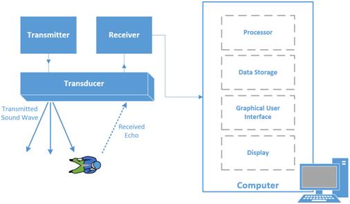
2.3.1 Block Diagram:

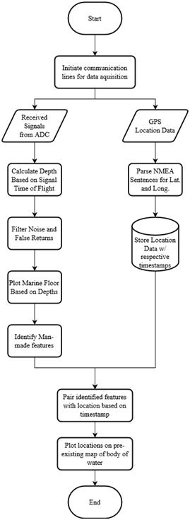
The figure below depicts a block diagram of the general system that will be implemented in order to collect data through the use of sonar in order to identify and visualize three dimensional objects underwater.

The system begins with the general transducer that will send and receive the sound waves that will be used to detect underwater objects. The raw resulting sonar recordings will then be processed using developed algorithms to obtain an image from the experimental data. Once an image is created, further image processing techniques will be implemented to identify object shapes and finally alert the user when such shapes are found.

3.0   Determining System Requirements

In this section, various factors that influence the final system design are discussed ultimately leading to the technical requirements necessary to ensure system functionality.

3.1   Wave Properties:

The properties of the wave transmitted by a sonar determine a large amount of what the sonar can locate. Some of the biggest trade offs to consider are resolution and distance. Higher frequencies have a higher resolution and thus can see smaller objects, but lower frequencies can see further into the water with less distortion. Since the sonar is focused around locating marine litter such as lobster traps, the resolution must be high enough to do this. Wave physics dictates that for a wave to locate any object, the wavelength must be smaller than the shortest side of the object. Most available lobster traps have 1” by 1” mesh sides (Robust) or 25.4mm by 25.4mm. Combining this with the speed of sound in water 1500 meters per second (Nieukirk), the speed equation of a wave to determine the minimum frequency needed.

? = ??

? = ?/?

?  =  1500/.00254  = 59???

?_????? > 59???

The next property to consider is the maximum frequency. The maximum frequency is less straightforward. As the frequency increases the absorption of the energy also increases. To get the wave to the target and back, the base energy of the wave must be higher. The deepest lobster traps tend to sit around 120 fathoms (McCarron) or 220 meters. At over 120 decibels, organic life can start suffering damage to hearing or organs immediately (CDC). Garmin, a common sonar brand, limits their loss to approximately 25 decibels at max range. Considering both of these factors, the absolute maximum decibel starting range is about 135 decibels. Garmin also shows that their trigger threshold for their sensors is approximately 110 decibels. Considering the maximum depth of 220 meters for lobster traps, a higher max depth of 250 meters should be
used. At this new max depth a distance of 500 meters must be covered. With a maximum loss of 25 decibels, the maximum frequency that can be used is around 200kHz

For the pulsing time to avoid interference, the previous signal would need to have been allowed to travel the full distance and back. The maximum range our sensor would be able to transmit is a 500 meter round trip. Since sound travels 1500 meters per second in water, a pulse can be transmitted at 3Hz without interference.

In conclusion the wave must: have a frequency between 7 and 200 kHz, pulse at 3Hz or slower, and have a returning sound pressure level of approximately 110 decibels

3.2  Transducer, Transmitter, and Reducer:

The orientation and setup of transducers is an important factor when considering a sonar setup. Generally due to the multidirectional nature of sonar, a linear arrangement of the transducers is almost always required. From the data provided in the Garmin spreadsheets (Garmin. Transducer Selection Guide. 10), most transducers have a trigger threshold of aproximently 110 decibels.

Lastly, though adding more transducers significantly increases accuracy of the sensors reading, having at least two transducers is a requirement to create a proper map of an area as it is not possible to map an area with only one transducer.

3.3   Data Processing Capabilities:

Once the transducer of the system is able to send and receive sound pulses, the next step in creating a functional object detection system will be to process and analyze the returned signals that reflect off of the target. As the data of a scan is collected it will be stored on board within a memory device of appropriate size. This will be discussed in further detail in the section below. The best place to store and process data will be on board. This must be done in order to provide immediate feedback to the user and alert them when the object they are searching for is detected. While in the past it may have been more beneficial to process large amounts of data off-board due to limitations in computing power, technologies have advanced enough where it will be possible to do all computations on a portable computer.

3.4   Data Storage:

While using the sonar device to scan underwater targets, recordings of the scans will be kept in order to assist in the visualization and processing of the received data. In order to keep the scanned data, it must be stored within the constructed sonar device. In order to determine the amount of data storage capability required for the device, multiple tests were done using various Garmin fishfinders. Detailed accounts of these tests can be found in the Background chapter of this report. Using the data from these tests, it was determined that the collected data files ranged from a two minute recording with a size of 4 MB to a four minute recording with a size of 20 MB. Additionally, Garmin’s website states that 15 minute recording uses about 200 MB of space (Garmin). In order to determine the approximate amount of data needed per minute of

recording, the ratio of each of these examples was determined, then the average MB per minute was calculated.

4 ?? ÷ 2 ??? = 2 ??/???

20 ?? ÷ 4 ??? = 5 ??/???

200 ?? ÷ 15??? = 13.3 ??/??��

(2 ??/??? + 5 ??/??? + 13.3 ??/???) ÷ 3 = 6.8 ??/???

For ease, the average will be rounded to 7 MB/min for future analysis. Although the actual size and complexity of future recordings is not yet known, the constructed sonar should have 1 GB of data storage availability. Based on the above analysis, this will allow for about 142 one minute recordings to be stored at once. Additionally, this will provide significant flexibility in how large and long the recordings can be. The data will be stored on an external drive within the sonar device’s processing system. This will allow the recorded data to easily be transferred when it comes time to analyze and process it. Finally, having a removable data storage device will permit the removal of recordings from the device in the case that additional tests beyond the 1 GB of available space become necessary.

3.5   Imaging Technologies:

In order for the final user to identify structures in the water, an imaging process will need to be implemented. Imaging sonars function by transmitting sound pulses and then converting the returned echoes into digital images (Soundmetrics). In most instances, a sonar image of an underwater object will very closely resemble an optical image of the same object.

Currently there are several products on the market today that are able to achieve this in a sonar system. These programs are either propretery, created by sonar marine electronic companies like Garmin, Humminbird, and Lowrance. There are open source programs available as well on platforms such as the Python language or MATLAB that can be used to gather and process any sonar data in order to create a final image of a scan. For this project, a combination of commercial products and open source files will be used to gather the raw data, clean and process it into a depth reading, visualize the marine floor, and then detect a manmade structure on the marine floor. Issues may be encountered when working with proprietary softwares of the transducers we choose to use. In order to work around this issue, a breakout box may be used with the receiver in order to detect the signals that have been sent from the transmitter and reflected from the marine floor back to the receiver. An amplification circuit should be used with a processor with accessible GPIO pins in order to send the ADC readings to the computer running the mapping software. Using the ADC readings, a program should be written that can calculate depths and eventually stitch together 2D images to create a 3D image of the marine floor in order to detect man made structures. The final object detection program should be able to be written in the Python language or MATLAB.

3.6   Localization Technologies:

A useful feature that this system should have is the ability to identify where in the world an interesting dataset is located in order for the user to return to that location at a later time if they desired. A data localization feature would also be useful to plot all interesting data points on a map of the region for easy analysis of the environment as a whole. In order to achieve this a global positioning system (GPS) module will be integrated into the overall system. Such a module will allow one to acquire National Marine Electronics Association (NMEA) data readings . The NMEA has developed standards for interfacing between various pieces of marine electronic information to ensure that all mariners are using the same information for consistency. Each line of data read from a GPS module contains a NMEA sentence which one could decode and parse for longitude, latitude, altitude, as well as date and time information. Using such a module with these communication standards will allow for our system to accurately track the position of its incoming data points.

3.7   Power:

Nearly all commercially available fish finders are powered by 12 volt batteries. Since the constructed sonar system will be based on a fish finder, a 12 volt battery will be used as the main power source as well. Once the final circuit diagram for the system is created, the exact power consumption required will be calculated. However, it is safe to assume that a 12 volt battery will provide enough energy to power the final system.

A 12 volt, 8 amp-hour battery will be used to power the system. The calculation for the stored watt-hours is detailed below.

?ℎ ∗ ? = ?ℎ 8?ℎ ∗ 12? = 96 ?ℎ

It is necessary for the power source to be in mobile form to allow the sonar device to be maneuvered around the water body. Using a 12 volt battery will permit this necessity.

3.8   Technical Requirements:

In the preceding sections of this chapter, the minimum technical attributes for a sonar device used in locating objects submerged in water were determined. A summarized list of these findings is detailed below.

• The sonar must be compatible with a removable, external data storage device.
  • The sonar must be able to be powered with a 12V battery.
  • The sonar transducer must be capable of side imaging and down imaging to further compare data collected using the two types of views.

Based on these requirements, a Garmin 73SV chartplotter display equipped with a CV52HW- TM transducer was selected. Some properties of this transducer are listed below.

• Traditional 24 degree by 16 degree beam dimensions
  • 12-pin connector
  • CHIRP, side imaging, and down imaging frequency of 455kHz or 800kHz
  • Down imaging and side imaging compatibility
  • Transmit power of 500W (RMS) / 4000W (peak to peak)
  • 7.1W power consumption
  • 2300ft maximum depth in freshwater
  • 1100ft maximum depth in saltwater

Each of these attributes meets the minimum requirements outlined. Additionally, the wide range of provided frequencies allows for further experimentation on data collection and processing.

The only requirement for the sonar display is that it is compatible with the provided transducer. This is why the Garmin 73SV was selected.

4.0   System Overview:

Overall, the final system will contain an electrical, software, and mechanical component. Working in conjunction with each other, these systems will be able to visualize the bottom of the aquatic environment in which they are scanning.

4.1   Proving System Feasibility:

In order to collect signals generated from the Garmin 73SV chartplotter, it was hypothesized that connecting a second transducer to an oscilloscope would detect the transmit and receive signals emitted by the transducer attached to the Garmin chartplotter. The below sections detail the setup, execution, and results of the tests performed.

As mentioned above, a Garmin 73SV chartplotter was used to complete the tests confirming that send and receive signals from one transducer can be observed by a second transducer. The provided Garmin chartplotter came equipped with a Garmin CV52HW-TM transducer. In order to complete the tests accurately, a second Garmin CV52HW-TM transducer was obtained.

Additionally, an oscilloscope and a Garmin breakout box were provided.

The purpose of a breakout box is to allow easy access to wire leads within the transducer, preventing the need to open the transducer. Using these leads provides access to signals produced by the transducer that can be interpreted as raw data. An image of the breakout box used, as well as the signal provided by each lead can be found below.

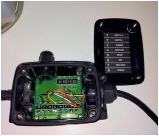
The numbers on the breakout box correspond to the following signals generated by the transducer.

1: Depth +

2: Depth –

3: Shield

4: Ground

5: Temperature

6: XID

7: SPD PWR (POSITIVE RECEIVE)

8: Speed (NEGATIVE RECEIVE)

First, the breakout box was connected to the first transducer. The oscilloscope ground was then connected to the grounding wire from the breakout box and the oscilloscope probe was connected to the Depth+ lead from the breakout box. Separately, the Garmin 73SV chartplotter was connected to a 12Vdc, 8Ah battery as well as the second transducer.

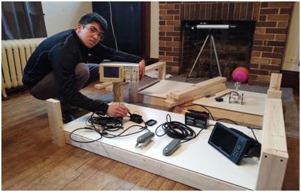
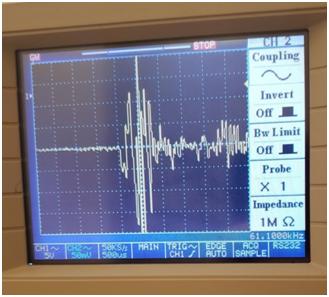
This entire system was then moved, and the two transducers were placed in a full bathtub. Since the purpose of these tests was to confirm our assumption that a second transducer could detect the signals transmitted and received by the first transducer, a bathtub was used so the tests could be completed in a controlled environment. Ideally, this would limit the amount of outside noise inhibiting signal reception. Once submerged, the transducer attached to the Garmin chartplotter was set to 200kHz. Various items were placed in front of the transducer in order to ensure data was being recorded correctly. Once this was confirmed, the oscilloscope was set to record Voltage Versus Time. Tests were then done to determine the time it took for the signal transmitted by the transducer on the chartplotter to be received by the second transducer.

After completing the tests, it was confirmed using the oscilloscope that we would be able to use a transducer to determine the time of flight of sonar pulses underwater. The first graph confirms the ability of our newly acquired transducer to detect the send and receive signals from our transmitter.

4.2   Electrical System Design:

The purpose of the electrical system is to detect the feedback from the sonar crystal and convert it into information the computer can decipher. Two different major circuits make up the electrical system design for the sonar. The first is a signal amplification circuit which takes the signal from the crystal, filters out any noise then converts the signal into readable information for the adc. The second portion of the circuit is the ADC. The ADC will need to take the converted signal in analog, convert the signal to digital, then inform the microcontroller when the signal is ready to be read.

4.2.1 Signal amplification Circuit:

• 4.2.1.1  Frequency and Voltage limitations:

The crystal that is acting as the receiver resonates at 200KHz. While resonating, the crystal has output between 40mV and 40 μV. The small voltage and high frequency of the incoming signal limits the number of viable transforms of the signal. The small voltage causes the greatest issue in how system noise must be handled. Normally, the small frequency range would make noise filtering with a band pass filter the easy solution. This cannot be done with the sonar crystal due to the small loss found within the pass range of the band pass filter. This is why an instrumentation amplifier was selected to filter out noise from the signal.

The instrumentation amplifier requires a differential input, which the crystal can provide. From the differential input, the noise can be negated by subtracting the negative of the differential input from the positive input. The largest issue the high frequency causes is in the operational amplifier. The operational amplifiers are sensitive to frequency. If the frequency gets too high the operational amplifier cannot switch its output fast enough to maintain a proper output.

Since the output of the signal will be most accurate using the full range of 0-Vdd range (0-12v) and the input is at its smallest 40μVpk, in total the entire circuit needs a gain of 150000 volts. This is broken into 3 stages using a gain of 100Av, 10Av, and 100Av. The second gain was lowered to keep the signals from hitting the output rails of the operational amplifiers as easily. This requires that the minimum gain bandwidth product of the circuit is 20MHz. The circuit is

also expected to swing between 0 and 12 volts with no issue. This requires a minimum slew rate

of 15V/μS.

• 4.2.1.2  Instrumentation amplifier:

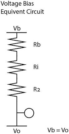
The instrumentation amplifier is broken into two stages. The first stage is a booster stage. This booster stage is important because it raises the signal’s voltage out of the range that noise can still significantly impact. The entire circuit only has a single supply. The issue that occurs from this is that the operational amplifiers cannot boost a signal into a negative value without a dual power supply setup. This can be fixed by providing a voltage bias to the operational amplifier. To allow the greatest range of signal amplification, a voltage bias of half Vdd (6V) is used for the bias.

This does create two small issues. The first issue is that the crystal is susceptible to high continuous voltage. To prevent damage to the crystal, the crystal was decoupled from the operational amplifier with a capacitor. The other issue is that the operational amplifier could lose the signal due to impedance from the voltage bias. The chosen operational amplifier has an internal resistance of 300KΩ, so to ensure the voltage bias does erase the signal, it must be separated with a minimum of 3MΩ anywhere the voltage bias is provided through a parallel connection. Anywhere a serial connection is used, a maximum of 3KΩ resistor should be used, though a 1KΩ resistor was commonly used instead

After the boost stage, the signal then transfers into a boosting and differential stage. Since our signals had been boosted equivalently to this point, the noise on both of them is still equal and cancels out during this stage. This stage is also given a voltage bias for the same single supply issue discussed earlier.

• 4.2.1.3  Boosting stage:

The final boosting stage makes use of a single inverting amplifier. The output from the previous stage is decoupled using a capacitor so that the signal can be voltage biased. The output from this stage gives a 0-Vdd with a bias at half Vdd signal.

• 4.2.1.4 Power:

The power for the circuit is broken into two very simple parts. The first is the 12 volt battery which provides Vdd for the circuit. The second part is a 6v zener diode resistor pair working as a voltage regulator to provide half Vdd for the voltage bias.

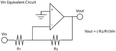
• 4.2.1.5  Circuit Analysis:

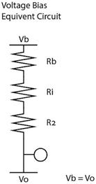
For the first boosting stage of the circuit, the circuit must be evaluated in two ways. The first way is for the 0 Hz DC bias voltage. The second is for the 200 kHz ac signal.

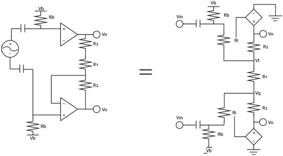
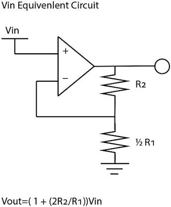
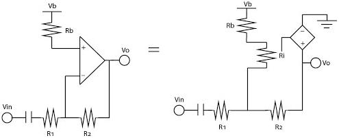
The voltage bias is unable to travel through the capacitor separating it from the ac signal. It is also unable to ground on R1 as the same voltage is on both sides of the capacitor. The capacitance of 1μf was chosen to provide the hard cutoff for dc signals needed for this design to work. This means the bias has one path through the operational amplifier. The only way for this path to give a stable output at the Vout is for Vout to be equivalent to Vb to prevent current from flowing through the operational amplifier.

The AC signal can travel through the capacitor and can ground on half of R1 due to the signals being  inverse. It is also unaffected by Rb due to the fact that Rb is ten times bigger than Ri and is in a parallel connection with Ri. Rb is 3MΩ, and Ri is 300kΩ. This means none of the signal is lost to Rb. This means it operates as a normal non-inverting amplifier in its superposition. R1 is 2kΩ and R2 is 100kΩ to provide a 100 times gain for this section.

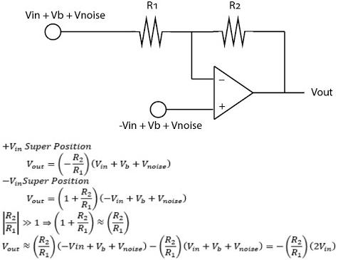
The next stage is the differential amplifier. As this stage is using two inputs, it is also best analysed with super positions. This stage relies on using a non-inverting amplifier as well as an inverting amplifier setup. It is also important in this stage that an equivalency is drawn between the formula (1+R2/R1) and (R2/R1). This means that for the best result the largest amount of boosting should be done in this section. This is not the case though as the working model uses a 10kΩ resistor for R2 and a 1kΩ resistor for R1. These provided the 10 times gain needed for this section but should have had 100 time gain.

Lastly, the final boosting stage is analyzed in a similar manner to the one above. It is broken into the voltage bias superposition and the ac signal superposition. It operates in the exact same way with the same limitations to the circuit above.

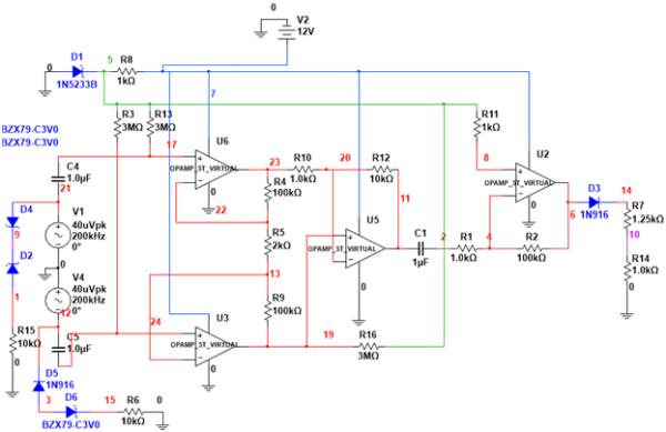
• 4.2.1.6 Final Circuit:

The image below depicts the final circuit using the components described above.

4.2.2 Transmit Signal Output:

It was discovered during testing that the transmit signal for the crystal would operate at around 30V. This signal was significantly higher than any feedback recorded. Due to this fact, a zener clipping voltage regulation setup was used so that anytime the voltage exceeded 3v or -3v, the voltage would travel down a different path and not through the amplification circuit. This path would then be connected to the microcontroller so that transmit signals could be read from another pin.

4.2.3 ADC incorporation Circuit:

The last part of the signal is setting up the signal for the ADC. The ADC can only read between 0V and 5V, so the output signal of the amplification circuit was run through a diode and a voltage divider to change the range from 0V to 12v with a 6v bias to 0V to 5V with a 2.5v bias. This new setup was then transmitted to the ADC to be converted for the microcontroller

4.2.4 Testing the circuit:

The circuit was provided with a 12V source and a 100KHz, 1V signal. This signal caused the output to swing between 0V and 12V out. The signal, when provided with 0V and an impedance on the input terminals, did also stabilize at the 6V output.

4.3   Software System Design:

The purpose of the software being implemented is to collect the incoming data from the ADC and ultimately obtain useful information for the end user based on voltage readings and the time between those readings. The end goal is to continuously determine the depth to the marine floor and locate marine objects underneath the data collection vehicle at all times. This depth data would then be visualized for the user and a trained algorithm will analyse the geometry of the marine floor structure in an attempt to identify any man made objects that may have been lost over time. Supplemental data will be collected from another device in order to tag all incoming data from the transducers with a geolocation which will be used to plot the location of a data capture session which would be useful to the end user if they wished to return to the exact location where a man made object of value may have been lost. All software features for this system were programmed in the versatile Python programming language.

4.3.1 Depth Visualization and Analysis:

• 4.3.1.1  Data Acquisition from ADC:

In order to visualize depths and perform analysis on underwater marine structures, voltage readings from the transducers were collected and interpreted. The approach that was taken to achieve this involved using an ADC to sample the send and receive sonar signals that are being passed through the amplification circuit. In the figure below, the wiring of the system is pictured.

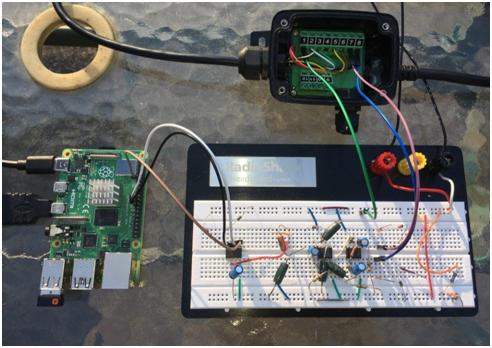
The white and black wires connected the data transfer pins and clock pins of the ADC to the raspberry pi. The brown wire was connected to the CONV pin of the ADC and controlled with an arbitrarily chosen GPIO pin of the raspberry pi. The green wire of the breakout box was connected to the ground of the circuit. The blue and purple wires of the breakout box were connected to the two input locations of the voltage amplifying circuit.

In order for the raspberry pi to receive these digital voltage readings, a reliable line of communication between the ADC and the raspberry pi was established since many data readings

will be processed every second. A data transfer system was set up using an SPI communication line. The SPI busses were enabled through the Raspberry Pi’s ‘sudo raspi-config’ command.

A Python program was written to collect the ADC data from the circuit. First the necessary libraries were imported. These were:

• RPi.GPIO – used to enable GPIO pin to toggle high/low for ADC functionality
  • binascii – used to translate raw data from ADC to human readable content
    • spidev – used to enable the SPI communication line and configure settings such as the number of bytes being read and the clock speed
    • time – used to created a precise timestamp for each data reading obtained from the ADC
    • csv – used to write all incoming data to a file for future analysis

After all libraries were imported, an SPI object was created using the spidev.SpiDev() function. Then parameters were created for the SPI object such as number of bytes to read and clock speed. Next a while-loop was initiated to start the data collection process. This loop started by setting a GPIO pin too low for the CONV of the ADC. Then a response of data was read using the spidev library. Next the CONV was set high. Finally the collected data was written to a new csv file with a precise time stamp. This timestamp will be used later to associate data points with GPS location which will be collected at the same time.

• 4.3.1.2  Interpreting ADC Readings to Depth Values:

Once a mode of communication was established, the next part of the software system was able to start interpreting the incoming voltages readings from the transmitter and receiver. First, the program looked for a transmit signal which was recognized by a large voltage reading as the passive transducer that the ADC is drawing readings from will detect the strong send signal from the powered transmitting transducer that is inches to the side of it. In order to determine what such a reading from the ADC would look like for this scenario, a test was conducted in the pool.

First the Garmin chartplotter system was connected to one of the transducers which was placed at the surface of the pool as seen in the image below.

The depth was able to be determined precisely using the Garmin chartplotter. The figure below shows that the depth of the pool relative to the transducers location was 7.5 feet. This number was then used to calculate the distance that a sonar pulse would travel 15 feet or 4.572 meters. The sonar speed of sound (1450 m/s) was then used to determine that it would take 0.003153 seconds for the transmitted pulse to be received.

This time of flight measurement was then used to determine the characteristics of the true received signal. ADC data was collected while the transducer remained in the same position.

Then, using the timestamps associated with the collected samples, the signal was easily identified. This was then used to identify when all other transmit signals were received in order to calculate depth.

Once a transmit signal was detected, a variable was initialized to a timer which started to count the time it takes for the signal to travel to the bottom of the marine floor and back to the passive transducer. When the signal is received and detected, the timer is stopped and the variable will now be equal to the time it took for the signal to travel from the boat, to the marine floor, and back to the boat. This value will then be used to calculate the depth at that point in the body of water being surveyed. This is easily done by using the speed of sound in water and multiplying that constant by the time elapsed variable. This is then divided by two as only the distance from the boat to the marine floor is important, not the distance to the bottom and back. The newly found depth value is added to an array data object which will be processed at a later time in order to create the profile visualization of the marine floor.

• 4.3.1.3  Filtering Noise and False Return Signals:

An important feature of the receive signal detection program involves being able to distinguish between the actual return from the transmit signal and false readings such as echoes of past transmits or noise that is present in the data collection environment. In order to combat against false readings and risk corrupting the final dataset, a feature was implemented that will disregard all readings that fall below a set threshold. This threshold value will be determined in a controlled environment to observe what the typical voltage value would be for the first return reading of a transmit signal so that values below this typical value can be labeled as either an echo of a past transmit or a reflection from other objects in the environment. The controlled testing environment will also allow for a noise floor to be determined. All voltage readings below this noise floor will also be disregarded when collecting readings from the ADC.

• 4.3.1.4  Processing Collected Depth Values:

The next piece of the software system takes in the previously created array of depth values that have been taken overtime during a depth acquisition session and visualizes it to create a 2D image of the marine floor that the boat has passed over. This was done by utilizing the Python

libraries NumPy and MatPlotLib. The program iterates through every index in the array that is passed in as the initial parameter, plots a point on a depth over time graph, and then connects each graphed point with a line to recreate the marine floor.

• 4.3.1.5  Detecting Man Made Objects:

The final component of the software system involves a program that analyzes the geometry of the line of the plotted ocean floor to determine if there are any man made objects on the marine floor. For the first version of this system, targets were attempted to be detected on the marine floor. In order to accomplish this, the program will first need to know what it should be looking for. In a controlled environment, a depth acquisition session will be performed with no targets present. The data will simply result in a flat line of the ocean floor being plotted. Several data inferences can be drawn from this dataset such as deviation in the Y axis of the points plotted over time, the slope connecting each depth point, and the rate at which the data points may be increasing or decreasing in the Y axis (the Y axis holds the measurement of depth while the X axis hold the measurement of time). Next, the same procedure will be performed with a target present on the ocean floor with minimum noise in the environment. The same data inferences will be recorded.

When a plot of the marine floor is produced, the target detection program will compare the plotted features to the features observed in an empty environment and when a target is present. The program will compare all points and slopes and look for common patterns indicating that a target is present. For example, the program may find that there are two instances in a depth plot where the Y axis changes suddenly twice, creating a square or rectangle shape. Based on the training data collected, the program can determine that a lobster pot has been detected and the end user will be notified.

4.3.2 Acquiring and Integrating Additional Data

While the system mentioned above is suitable for quick analysis of whether a man made object is detected in an environment, it would be useless if the user is unable to recover the items right away and will need to return to the location of the detected object at another time. In order to enable the end user to do so, a GPS module will be implemented which will log latitude and

longitude data while the sonar system is sending pulses and depth readings are being calculated. In order to obtain data from the GPS module, a serial communication line was set up between the GPS and the raspberry pi by using the hardware UART GPIO pins on the computer. This is achieved by first configuring the raspberry pi to enable hardware communication through serial and disabling shell and kernel messages. Next, the config file of the raspberry pi is edited to enable UART for all users. This must be done with administrative privileges by prepending the edit command with ‘sudo’. Next the libnfc library is created to allow userspace access to NFC devices. After a few more minor changes to configure the raspberry pi, the libnfc library is built and the GPS module is ready to use for data collection.

To read the data coming in over the opened line of communication, the following code snippet can be run.

import time import board import busio

import adafruit_gps import serial

data_in = serial.Serial(“/dev/ttyS0”, baudrate=9600, timeout=10

      while(1):

while GPS.inWaiting()==0:

Pass NMEA=GPS.readline() print (NMEA)

As depth readings are being calculated they will be paired with an accurate location data point that the GPS module will constantly be read from the raspberry pi computer. In this case, a new data object will be created which consists of an array of arrays which is demonstrated below.

[[depth_data_0, gps_data_0], [depth_data_1, gps_data_1], … [depth_data_n,

gps_data_n]]

In order to save time and system resources, the raw data string from the GPS module will be left as is until the program has collected all data points and needs to plot the points on a map. The raw GPS data will be brought into the data object as a NMEA string. This standardized format is composed of many characters and numbers that are meaningless to the human eye. A sample of one GPS reading consisting of its NMEA sentences are pictured below.

$GPGGA,123519,4807.038,N,01131.000,E,1,08,0.9,545.4,M,46.9,M,,*47

$GPGSA,A,3,04,05,,09,12,,,24,,,,,2.5,1.3,2.1*39

$GPGSV,2,1,08,01,40,083,46,02,17,308,41,12,07,344,39,14,22,228,45*75

$GPRMC,123519,A,4807.038,N,01131.000,E,022.4,084.4,230394,003.1,W*6A

$GPGLL,4916.45,N,12311.12,W,225444,A,*1D

$GPVTG,054.7,T,034.4,M,005.5,N,010.2,K*48

$GPWPL,4807.038,N,01131.000,E,WPTNME*5C

$GPAAM,A,A,0.10,N,WPTNME*32

$GPAPB,A,A,0.10,R,N,V,V,011,M,DEST,011,M,011,M*3C

$GPBOD,045.,T,023.,M,DEST,START*01

$GPBWC,225444,4917.24,N,12309.57,W,051.9,T,031.6,M,001.3,N,004*29

$GPRMB,A,0.66,L,003,004,4917.24,N,12309.57,W,001.3,052.5,000.5,V*20

$GPRTE,2,1,c,0,W3IWI,DRIVWY,32CEDR,32-29,32BKLD,32-I95,32-US1,BW-32,BW- 198*69

$GPXTE,A,A,0.67,L,N*6F

$GPMSK,318.0,A,100,M,2*45

Clearly none of this data will make any sense to the end user when determining the location of their measured depth values. However, a python script will be able to quickly parse the NMEA sentences for the latitude and longitude at each given point in time. This will be the most important piece of information needed to be uncovered from the NMEA raw data, but other information that could be useful includes time and velocity. The code snippets below allow for one to extract only the latitude and longitude data and convert them into usable coordinates.

Once the usable coordinates have been obtained, the data points indicating a lost target can be mapped on a navigable map of the area for the end user to reference in the future. This can be accomplished using Google Earth and a KMZ wrapper .xml file. A skeleton version of this wrapper can be seen below. A function will be created to take all latitude and longitude values, pair them into their respective coordinates, and then add them to the KMZ file where there is a space between <coordinates> and </coordinates>. A new KMS file will be saved on the system once all coordinates have been added. The end user can then easily upload this file to Google Earth and they will be able to see where they traveled exactly when they were collecting depth data in order to recover lost targets.

<?xml version=”1.0″ encoding=”UTF-8″?>

<kml xmlns=”http://www.opengis.net/kml/2.2″>

<Document>

<Style id=”yellowPoly”>

<LineStyle>

<color>7f00ffff</color>

<width>4</width>

</LineStyle>

<PolyStyle>

<color>7f00ff00</color>

</PolyStyle>

</Style>

<Placemark><styleUrl>#yellowPoly</styleUrl>

<LineString>

<extrude>1</extrude>

<tesselate>1</tesselate>

<altitudeMode>absolute</altitudeMode>

<coordinates>

</coordinates>

</LineString></Placemark>

</Document></kml>

In the future, another function may be created that will automatically upload the KMZ file to Google Earth directly without any interaction from the end user.

4.4 Mechanical System Design:

The purpose of the mechanical system is to provide a platform for the transducers, chartplotter,
electrical system, and software system to be combined. This will allow the overall components to
work in conjunction with one another while floating on the water being used for testing. Two
different mechanical systems were developed for use in different testing situations. One was
designed to be implemented as a stationary device used in areas where motion is not required.
The second was designed to be a mobile application in order to aid in the mapping of the testing
environment floor.
4.4.1 Stationary Application:
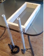
A bracket was designed and built to be able to fix the location of the transducers when doing
experimental tests in controlled environments such as a pool or bathtub. In turn, this would allow
decreased variance in transducer motion during testing allowing for more accurate results. The
bracket was built using wood boards, PVC pipes, and clamps. The image below shows the ideal way 

to position the bracket. Ideally, the base would be placed on the edge of the experimental
waters, such as a pool, which the transducers were submerged in the waters below.

The individual pieces used in the construction are as follows:
● 2, 24 inch 2×4
● 2, 12 inch 2×4
● 2, 12 inch 1.5 inch ID PVC
● 2, 28 inch 1 inch ID PVC
● 4, 1.75 inch to 2.75 inch pipe clamps
The 2x4s were screwed together as depicted above. A single hole was drilled in each of the 12
inch PVC pipes 2 inches from the bottom. Holes were drilled every 6 inches in the two 28 inch
PVC pipes to allow the transducers to be raised or lowered to various depths depending on the
water level of the testing location. A transducer was then attached to each of the telescoping
PVC systems. Finally, the remaining two pipe clamps were attached to a 2×4 using a single
screw. These clamps were then used to attach each of the systems to the platform base.
In order to counteract the fact that the transmitted signals from each of the transducers may come
out of the transducers at slightly different locations or angles, the bracket was designed to have
multiple degrees of freedom for each of the PVC-transducer systems. This way the transducers
can be rotated around the x, y, or z axis in order to find the optimal location of signal emittance
from each of the transducers. The purpose of finding this location is to gain send and receive signals between the two transducers resulting in the most accurate and clean experimental data.
The images below show the three degrees of freedom designed into the circuit system. 

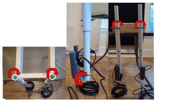
For the picture on the left, the PVC-transducer systems were attached to the 2×4 using the pipe
clamps to allow for this range of motion. The pipe clamps can be loosened and the PVC pipes
rotated in order to find the optimal transmission location of the transducers about the respective
axis.
For the picture in the center, the mounting brackets provided with the transducers allow for
rotation about the axis through the center of the bolt pictured. In this case however, the
transducers are only able to be rotated from the position shown until the point where the bracket
interferes with the PVC pipe.

The picture on the right depicts the final degree of freedom for the bracket system. A single
screw was used to attach the pipe clamp to the 2×4 so each individual PVC-transducer system
could be rotated independently.
Overall, the transducers were attached to separate PVC systems as the optional transmission
location is likely different for each of them. With separate attachments, each can be moved
independently of the other until the best quality testing data is generated.
In order to confirm the functionality of the bracket. Two main analyses were conducted. First,
the shear stress on the screws attaching the top pipe clamps to the 2×4 was calculated and
compared to the shear strength of steel. For this problem the total weight of the two PVC pipes
and transducers were modeled as a single force acting in shear on the screw. The weight of the
pipe bracket attaching the transducer to the PVC was considered negligible. The analysis was
completed only for a single PVC-transducer system under the assumption that the forces acting
on each would be the same.
Shear Stress Calculation:
Step 1: Total Weight of PVC and Transducer:
Garmin CV52HW-TM Transducer: From website: m = 1.13kg
12in 1.25in ID PVC:
ID = 1.25in = 3.175cm; OD = 1.66in = 4.216cm; ρPVC = 1.45g/cm3
; h = 12in = 30.48cm
V = πh(r1
2
– r2
2
) = π*30.48cm(2.108cm2
– 1.588cm2
) = 184.03cm3
m1 = V*ρPVC = 184.03cm3
* 1.45 g/cm3 = 0.267kg = 0.589lbs
28in 1in ID PVC:
ID = 1in = 2.54cm; OD = 1.315in = 3.34cm; ρPVC = 1.45g/cm3
; h = 28in = 71.12cm
V = πh(r1
2
– r2
2
) = π*71.12cm(1.67cm2
– 1.27cm2
) = 262.75cm3
m1 = V*ρPVC = 262.75cm3
* 1.45 g/cm3 = 0.381kg = 0.840lbs
Total Mass of Each PVC-Transducer System: 1.13kg + 0.267kg + 0.381kg = 1.778kg = 3.9lbs

Step 2: Free Body Diagram:

Step 3: Shear Stress Calculation:

#6 Screw Diameter = 0.0035m; Shear Strength of Steel = 200MPa
F = m*a = 1.778kg * 9.81m/s2
τ = (4F) / π(d)2 = (4*17.44N) / π(0.0035m)2 = 1.81MPa
FOS = τMAX / τ = 200Mpa / 1.81 MPa = 110.5
From the above analysis, it proved that the shear stress acting on the mounting screw in each
PVC-transducer system is very small compared to the shear strength of steel. As a result, it can
be assumed that the single screw provides enough support for the system.
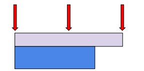
The second portion of analysis done revolves around the positioning of the bracket on the edge
of the experimental waters. Ideally, the weight of the rectangular 2×4 base would provide enough
counterbalance for the PVC-transducer system on its own without requiring a person to stand on
it. This step in the analysis seeks to calculate how much of the 2×4 base must be on the edge to
prevent the PVC-transducer system from falling into the water.
Static Analysis:

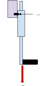
Step 1: Free Body Diagram:

In the above diagram, only one half of the entire bracket system was modelled, once again
assuming that each side has identical forces acting. F1 represents the force caused by the weight
of one half of the 12inch 2×4 in the back of the bracket base. F2 represents the force caused by
the weight of the 24inch 2×4. The force F represents the weight of the PVC-transducer system as
identified in the shear stress calculation. Point A represents the fulcrum between the pool edge
and the bracket base. r represents the distance between the pool edge and the end of the bracket.
The mass of the second 12inch 2×4 was considered negligible as it will be very close to the
fulcrum, thus providing little to no moment on the system as a whole.
Step 2: Force Calculation:
2×4 Data from Home Depot: 96in (2.44m) = 9lbs (4.08kg)
4.08kg/2.44m = 1.67kg/m
0.610m * 1.67kg/m = 1.02kg (mass of 0.610m section)
F2 = m * a = 1.02m * 9.81m/s2 = 10N
0.1525m * 1.67kg/m = 0.254kg (mass of half of the 0.305 section in the back)
F1 = m * a = 0.254m * 9.81m/s2 = 2.5N
F = 17.44N

Step 3: Moment Analysis:
The moment analysis below was done to calculate the minimum value of r where the force F
would not tip the system into the testing water.
2.5N(0.610m – r) + 10N(0.305m – r) > 17.44N(r)
1.525Nm – 2.5r + 3.05Nm – 10r > 17.44r
4.575Nm – 12.5r > 17.44r
4.575Nm > 29.94r
0.153m > r
Therefore, as long as the edge of the brack base does not overhang the edge of the testing water
by greater than 0.153m or 6 inches, the base will provide enough counterweight to hold up the
PVC-transducer systems.
4.4.2 Mobile Application:
For the mobile application of the designed sonar, a floatation device was constructed in order to
support the chartplotter, circuit, and transducers. This device will allow these parts to be buoyant
in the testing waters in order to move the system above various targets in the experimental water
body. Ideally, when this is functional the motion of the platform will serve as the third dimension
for target visualization. This device was constructed using mostly PVC piping along with a
wooden floor and foam walls to further protect the onboard devices from getting wet during
motion.

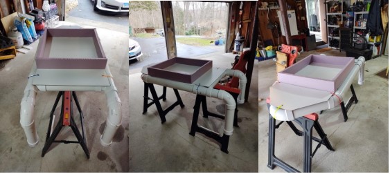
                                                                   Figure 29: Buoyant Platform

The majority of PVC piping was used to construct the base of the boat. Two pieces of 3in by
14in PVC were attached perpendicular to the base platform in order to allow the transducers to
be fixed to the platform underwater.
The PVC portion of the platform is what was used to make it actually float. Each joint was
sealed with a waterproof PVC adhesive in order to prevent water from filling up the pipes and
ultimately sinking the platform. The platform was constructed using 3in ID PVC piping cut to
the lengths below. For the purpose of future calculation, the volumes of each segment are
included as well. Since the volume used to calculate buoyancy refers to the sealed volume of the
PVC cylinder, the formula V = π*r2
*h was used. For the 3in PVC, the radius of the outer
diameter, 0.0445m (1.75in) was used.

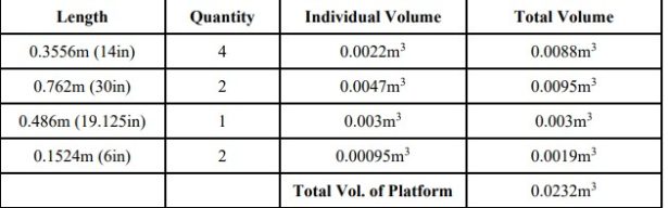
                                                                  Table 1: Volume of Buoyant Platform

Next, the mass of each length of PVC piping was determined for future use in analysis. For this,
it was assumed that 3in PVC pipe has a mass of 2.21kg/m. For each segment, this number was
multiplied by the length to determine the mass of each piece.

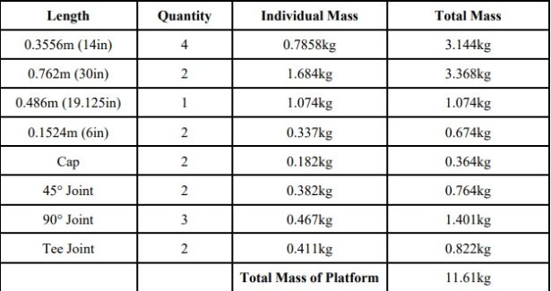
                                                                   Table 2: Mass of Buoyant Platform

For the calculation of the total volume of the buoyant platform, the volumes of the joints were
considered negligible as the pieces of piping generally fit into the joints very deep. Additionally,
for calculation purposes, the weight of the floor and walls added later were ignored.

Although it was observed that the platform would float when it was placed in the testing
environment, analysis was done to confirm this. Based on the total volume, the maximum
buoyant force was determined assuming the entire body was submerged. Then, this was
compared to the total gravitational force acting on the platform due to its total mass. In the
formula below Fb is the buoyant force, Vs is the submerged volume, D is the density of water,
and g is the gravitational constant.
Buoyant Force: Fb = Vs * D * g = 0.0232m3
* 1000kg/m3
* 9.81m/s2 = 227.88N
Gravitational Force from Mass: 11.61kg * 9.81m/s2 = 113.89N
Since the force coming from the mass of the boat, 113.89N, is less than the maximum buoyant
force, 227.88N, it was confirmed analytically that the boat will float.
Next, the estimated actual buoyant force acting on the boat was calculated. The image below
shows the boat in water prior to attaching the floor and walls.

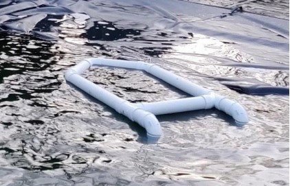
                                                                        Figure 30: Boat in Water

From this, it was estimated that the entirety of the 14in pipes in the back and one third of the
14in pipes in the front were submerged naturally. This was used to calculate that volume of material submerged. The actual buoyant force was then compared to the maximum buoyant force
to see if the boat was large enough to support the circuit, chartplotter, and transducer.
Submerged Volume: (2*0.0022m3
) + (0.33*(2*0.0022m3
)) = 0.00585m3
Buoyant Force: Fb = Vs * D * g = 0.00585m3
* 1000kg/m3
* 9.81m/s2 = 57.39N
227.88N – 57.39N = 170.49N of maximum buoyancy to spare
From this calculation, 170.49N of force, or 17.38kg of mass, could potentially be added to the
platform before it would be entirely submerged. Next, the force added by the transducers and
chartplotters was determined to see if it was less than the maximum remaining force. Due to its
small relative mass, the mass of the circuit was ignored.
From Garmin: mchartplotter = 0.77kg, mtransducer = 2.26kg
F = (0.77kg + 2*2.26kg)*9.81m/s2 = 51.89N
From this analysis, the mass of the transducers and chartplotters would only add an additional
51.89N of force to the boat which is well below the maximum capacity. As a result, it is
confirmed that the platform will be able to support the system.
For the final aspect of the mobile platform, a cranking device was created. The purpose of this
device is to attach to the front of the boat and then be placed on the edge of the testing
environment. When turned on, this device would pull the boat with the attached system in a
straight line across the water body at a constant speed. This constant speed would be used in the
visualization program to create a third dimension. The device can be seen below. 

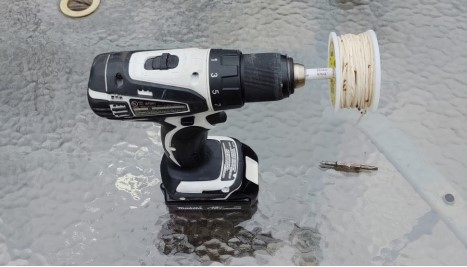
                                                                      Figure 31: Boat Pulling Apparatus

By using the drill, enough power would be supplied in order to adequately pull the boat across
the testing environment. To first determine the desired speed, the torque limiter on the drill was
set to 1N*m to ensure that if the boat started to go too fast, the drill would prevent it from getting
damaged. Within this range, various speeds were tested to determine which one pulled the boat
at a constant speed and kept it level. Once this was visually determined, an indentation was made
on the trigger of the drill so the speed could be recreated for testing purposes.
The primary calculations done using the cranking device revolved around the assumption that as
the line continually wrapped around the spool, the speed of the boat would be impacted as a
result of the increasing circumference. To determine the results of this assumption, the diameter
of the spool was measured when the line was fully wrapped around and when the line was
extended to the boat’s position across the pool.
Spool Diameter with Total Amount of Line: 6.87cm
Spool Diameter with Boat on Opposite End of Pool: 6.37cm
When the boat was on the other side of the pool, only a 0.5cm difference was observed in the
diameter of the spool.

Next, the average boat velocity across the pool was determined. To do this, the length of the pool
from the tip of the boat to the opposite end was measured. The boat’s motion from one end to the
other was timed, and the results are outlined in the table below. The formula
Velocity = Distance / Time was used to calculate the velocity.

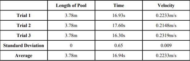
                                                                      Table 3: Boat Velocity Calculations

The numbers generated in this test not only provided the average velocity of the boat, but also
confirmed that using the indentation made on the drill trigger pulled the boat along the water at
generally the same rate. Next, the rotations per minute of the spool during the time the boat was
being pulled was determined.
Revolutions of Spool per Movement Across Pool = 17.75
Average Time = 16.94s
RPM = 17.75 / 16.94s = 1.05RPM
Finally, to determine the influence of the changing spool diameter on the speed of the boat, the
time was recorded between every full revolution of the spool as the boat was pulled across the
pool. Two trials were completed, and the raw data from these trials is outlined in the table and
graph below. For the graph, only data up to revolution 17 was used.

5.0 Conclusion:

Upon completion of this project a prototype for a depth finding and underwater object detection
system was created. A custom circuit was designed and built to detect and amplify received
sonar pulses underwater. An ADC that was incorporated into the circuit allowed for data samples
to be collected on a computer. This computer ran software to collect data samples from the
circuit and then calculate the depth at each point in time. Additionally, GPS location data was
collected on the same computer system allowing the final user to identify where depth data was
collected. A mechanical testing device and floatation apparatus was constructed allowing for inwater testing, experimentation, and data collection. The floatation device was equipped with a
custom cranking device to maneuver the device over a body of water at a constant rate creating
the ideal environment for data acquisition.

6.0 Future Work:

For future iterations of this system, students should focus on the following:
● Moving everything onto the boat in a watertight casing
For the tests performed in this project, the raspberry pi, provided chartplotter, amplification
circuit, and power source were kept outside of the water body used for testing. However, in the
final version of this product all of these would be included on the floatation device. This would
provide a single source for underwater 3D data collection without having to rely on having
access to shore. Additionally, the testing environment used in this project was short enough to
allow for these items to be kept on shore. Future iterations should be able to freely range
throughout a much larger source of water. Therefore, an important future part of this project is to
include a waterproof casing for all of these items when they are on the floatation device.
● Implementing underwater object detection program
A useful feature to the end user would be an automated way to determine if a manmade structure
located on a marine floor was identified during a depth finding scan. This could be done by
performing depth finding scans in a controlled environment of manmade objects like boxes or
crates and then using the geometries of the plotted marine floor to isolate these man made
structures as they will have orthogonal geometries.
● Linking GPS to object detection
Another useful feature to the end user would be the ability to localize all identified man made
objects during a depth finding scan. This could be easily implemented by comparing the
timestamps of the ADC depth data with the timestamps of the GPS data. If a man made object is
detected the program could look up what ADC readings are associated with those depth readings,
find the timestamp attributes for these data points, and then use this timestamp value to find the
GPS data that was collected at that exact point in time.
● Providing a notification system when an object is detected

An intuitive user interface could also be implemented in order to make data presentation easy to
understand by those who may not be familiar with the research tools used in this project. Such a
UI could consist of a simple notification that would send a message to the user via sound or light
to notify that a man made object was detected on the ocean floor.
● Perform marine floor testing in larger bodies of water
In order to confirm that this system will work in a real world environment, future iterations
should be tested in larger and deeper bodies of water. While controlled environments are
desirable research and development, they do not provide the conditions that will be encountered
if such a product were to be used commercially in ocean, river, or lakes.

 

Source: Underwater 3D Data Collection