Build a Raspberry Pi Zero cluster with MPI (Message Passing Interface). Employ parallel computing to discover all prime numbers under 100 million in approximately 24 seconds!
Introduction
Raspberry Pis offer an excellent platform for learning programming and experimentation. The Raspberry Pi Zero, being affordable and compact, might seem limited with its single core and 512 MB of memory in today's world of high-speed, multi-core computing.
Nevertheless, the saying “many hands make light work” rings true! Here lies an educational and enjoyable Raspberry Pi Zero project.
This project demonstrates how to create a cluster of Raspberry Pis, employing the “divide and conquer” strategy to leverage multiple devices collaborating together, producing results far beyond what a single computer could achieve. Through parallelization, adding more Pis further enhances overall performance.
MPI (Message Passing Interface) stands as the prevalent standard in parallel computing, boasting various implementations like MPICH and OpenMPI, among others.
Within this project, we will:
– Assemble a basic two-node cluster
– Gain an introduction to MPI and parallel programming concepts
– Execute sample workloads (such as finding prime numbers below a certain value) to compare execution times between single-node and parallel (2-node) scenarios, deriving insights from the comparisons.
Setting up the Cluster
Case:
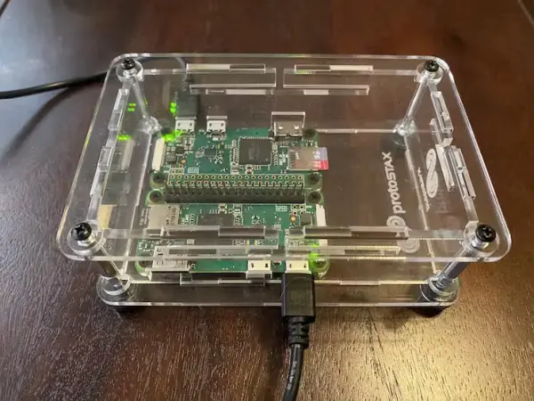
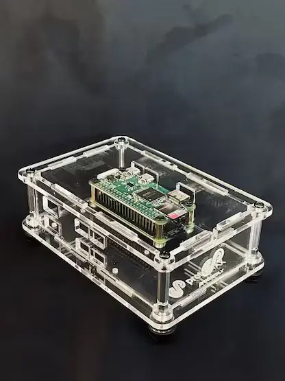
In this demonstration, I am establishing a cluster consisting of two nodes. To achieve this, I am utilizing the ProtoStax Enclosure specially crafted for Raspberry Pi Zero, capable of housing and positioning two Pi Zeros adjacent to each other, as illustrated in the image below.
It possesses a vertical clearance of 1.2 inches internally, providing ample space for a pHAT or Bonnet. Consequently, you can arrange 4 Pi Zeros in a stacked formation, 2 by 2.
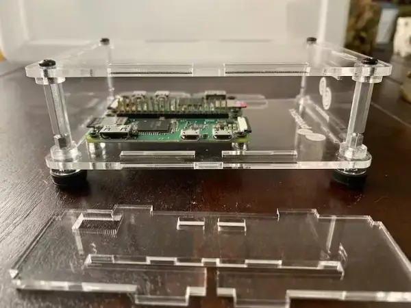
When arranging 4 Raspberry Pi Zeroes in this configuration, you have the option to omit the longer sidewalls, enabling access to the USB and power ports for all 4 RPis. The extended sidewalls have USB and power cutouts specifically designed for each Pi Zero. Refer to the illustration below for clarification.
Alternatively, the ProtoStax Cluster Kit designed for Raspberry Pi Zero offers a solution. It includes modified side panels for the ProtoStax Enclosure intended for Raspberry Pi Zero. These panels come with specific cutouts tailored for accommodating 4 Pi Zeros. This arrangement allows you to stack and safeguard 4 Raspberry Pi Zeros while maintaining protective side walls.
Networking:
In parallel computing, cluster computers necessitate communication among themselves. This interaction can be facilitated through Ethernet, which can either be wired or wireless.
In the context of my demonstration, I employ the wireless LAN capability of the Raspberry Pi Zero W for inter-cluster communication. Depending on the demands of your workload, involving substantial data transfers and extensive node-to-node communications, utilizing dedicated wired connections equipped with greater throughput might be more suitable. For instance, employing a Gigabit Ethernet switch and establishing wired connections among the Raspberry Pis could be a viable option. In such a scenario, transitioning to a more fitting Raspberry Pi model, such as the newer 4B that features a Gigabit Ethernet port for wired communications, would be advantageous.
However, for our specific workload involving prime number calculation, where extensive data transfer and communication aren't major concerns, the wireless connection suffices.
If you're unfamiliar with preparing your Pi for wireless communication, numerous online resources are available to guide you through the process. In my setup, I simply utilized a basic DHCP setup with my home wireless router and configured it to allocate the same reserved IP address to each Pi consistently.
Preparing the Pis
The initial step involves ensuring that all Pis, or in the case of a 4-node setup, all 4 Pis, are operating on the same OS version and are updated to the latest software version. This step is crucial to avoid potential communication problems among nodes running different software versions.
For my setup, I've installed the most recent version of Raspberry Pi OS.
After ensuring uniformity in OS versions, the next task is to configure the nodes to enable seamless communication between them. Among the nodes, one serves as the master while the others act as client nodes (also referred to as slave nodes). The master node will establish connections with each node in the cluster, and each client node must establish communication with the master.
To achieve this, we'll implement ssh key-based authentication for secure and efficient communication between the nodes.
We'll generate ssh keys using
ssh-keygen -t rsaand then distribute the public keys to the different hosts using
ssh-copy-id <username@hostip>The public keys need to be copied from the host to all the clients (so run the above command on
On the host computer, identify and allocate the client IP address for every client. Ensure communication from each client to the host (no need to manage file transfers between client machines). Next, proceed with the installation of MPI on each node. Specifically, we'll install MPICH and the MPI4Py Python bindings for MPI.
sudo apt install mpich python3-mpi4pyTesting your setup
Run this on each node
mpiexec -n 1 hostnameExecuting the command “hostname” on that particular node will yield and display the result.
Retrieve the IP addresses of all your nodes by utilizing the “ifconfig” command (refer to the Networking section above).
Subsequently, execute this command on your master node:
mpiexec -n 2 --host <IP1,IP2> hostnameThe command mentioned executes the ‘hostname' command on the specified nodes and displays the outcomes.
If you've reached this point, fantastic! Everything is in order, and you're all set to proceed!
A Bird's Eye Look at Parallel Computing
Here's a concise introduction to parallel computing and its fundamentals. It's more akin to viewing from an airplane at 30,000 feet than having a detailed bird's-eye perspective.
After creating a Raspberry Pi Cluster, there are various ways to maximize its potential or optimize a single Raspberry Pi further. Techniques like multi-threading enable the CPU to seemingly execute tasks in parallel. For instance, one thread could use the CPU while another waits on input/output, dividing the CPU's time among these threads.
On a multi-core processor, such as the Raspberry Pi 4B, actual parallelism occurs by simultaneously running multiple processes. Leveraging communication models like MPI allows running processes on different physical nodes, expanding parallelism beyond a single node (even within a single node). As an illustration, MPI is employed here to parallelize the task of identifying prime numbers below a specified value, say all primes below 100 million.
Effectively utilizing parallel computing involves breaking down a problem into multiple tasks, each capable of independent parallel execution. These tasks need to run concurrently and autonomously. Subsequently, combining individual outcomes is necessary to yield the final result, requiring communication for coordination.
MPI provides communication paradigms facilitating task decomposition, execution, communication, and result aggregation.
For better comprehension, let's explore an example related to finding prime numbers. However, before delving into that, let's briefly introduce MPI.
A Brief Introduction to MPI
A comprehensive MPI tutorial requires more space than what's available here, so I won't attempt it. Yet, I'd like to offer a glimpse of an MPI program—a sort of “Hello World” or “Blinking LED” equivalent—hoping it sparks your interest for more.
In C, the process begins with MPI_Init to initialize inter-process communications. At the program's conclusion, you utilize MPI_Finalize(). In between these calls, you execute the tasks of your parallel algorithm. Additionally, you can employ MPI elements such as size (indicating the cluster's node count), rank (defining your position in the cluster, acting as your cluster ID), and name (providing the node's name).
#include <mpi.h>
#include <stdio.h>

int main(int argc, char *argv[])
{
    int size, rank, len;
    char name[MPI_MAX_PROCESSOR_NAME];
#if defined(MPI_VERSION) && (MPI_VERSION >= 2)
    int provided;
    MPI_Init_thread(&argc, &argv, MPI_THREAD_MULTIPLE, &provided);
#else
    MPI_Init(&argc, &argv);
#endif

    MPI_Comm_size(MPI_COMM_WORLD, &size);
    MPI_Comm_rank(MPI_COMM_WORLD, &rank);
    MPI_Get_processor_name(name, &len);

    printf("Hello, World! I am process %d of %d on %s.\n", rank, size, name);
    MPI_Finalize();
    return 0;
}
The same code in Python is a little shorter, because the bindings take care of some of it.
#!/usr/bin/env python
"""
Parallel Hello World
"""
from mpi4py import MPI
import sys

size = MPI.COMM_WORLD.Get_size()
rank = MPI.COMM_WORLD.Get_rank()
name = MPI.Get_processor_name()

sys.stdout.write(
    "Hello, World! I am process %d of %d on %s.\n"
    % (rank, size, name))
Here is the sample output that I got:
$ mpiexec -n 2 --host 10.0.0.98,10.0.0.162 python3 mpihelloworld.py
Hello, World! I am process 0 of 2 on proto0.
Hello, World! I am process 1 of 2 on proto1.
Ok, how do we go from there to running some task/algorithm in parallel? Read on!
Computing Prime Numbers
To start, let's revisit the concept of prime numbers. These numbers can only be divided by themselves and 1, excluding any other number. Examples of prime numbers include 2, 3, 5, 7, 11, and 13.
The intriguing properties of prime numbers serve as valuable components in modern cryptography. If you're keen on exploring their applications, I've provided a reference at the end for your further understanding. In essence, contemporary encryption techniques rely on high-level mathematics. While it's relatively simple to multiply two large primes and obtain a significantly larger number, the reverse process of deducing the two original primes from a large number presents a far more complex challenge. Calculating primes up to substantial numbers is not only an engaging pursuit but also holds practical significance, as evident from cryptographic applications.
Our current endeavor involves identifying all prime numbers that are smaller than a specified number. For instance, the primes below 20 encompass 2, 3, 5, 7, 11, 13, 17, and 19.
Consider the scope of identifying primes under 10,000 or even below 1,000,000. It's evident that manual calculations are infeasible, necessitating the utilization of computational power to tackle this challenge.
The Brute Force Way
Determining if a number, denoted as N, is a prime involves dividing it by all numbers from 2 to N-1 and verifying if the remainder is zero (0). If none of these divisions yield a remainder of zero, then the number is considered a prime.
To identify primes within a specified range, each number within that range undergoes a similar primality test as described earlier. Any discovered primes are duly recorded.
Now, let's delve into the parallel algorithm's functionality. How does it function in this context?
The parallel algorithm enables the task to be efficiently divided and distributed. Each node takes on a designated portion of the given range (for instance, if the range is 1000, one node handles numbers from 2 to 500, while another addresses numbers from 501 to 1000). Every node then conducts the primality test within its assigned range and returns the results.
The master node orchestrates the process by consolidating the outcomes generated by individual nodes, presenting a unified summary to the user.
Using MPI (Message Passing Interface), each node can ascertain its rank within the cluster. This information helps nodes determine their allocated range of numbers for processing.
In the ‘prime.py' example I'm referring to, the distribution method may vary slightly, but the fundamental principle remains the same: dividing the task among nodes to expedite computation.
# Number to start on, based on the node's rank
start_number = (my_rank * 2) + 1
for candidate_number in range(start_number,
end_number, cluster_size * 2):
The rank assigned is either 0 or 1, given the presence of two nodes. Consequently, the start_number assumes the values 1 or 3. As the cluster comprises 2 nodes, the iteration increment is set to 4. Consequently, all multiples of 2 are excluded from processing, showcasing a slight enhancement over the least efficient brute force approach that tests all multiples of 2. In this strategy, within a range of 1000 numbers, each node handles approximately 250 numbers.
mpiexec -n 1 python3 prime.py <N>Running it on two nodes is as follows:
mpiexec -n 2 --host <IP1,IP2> python3 prime.py <N>where N is the number up to which we want to compute primes.
The primary node collects the arrays of prime numbers from each individual node, amalgamates them, and then presents the combined results.
Executing this process within a cluster of just one node is essentially identical to performing it on a solitary node, operating as a non-parallel algorithm.
Results
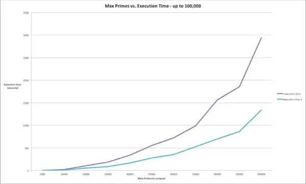
I conducted an experiment involving prime number computation from N=1000 up to N=100,000, increasing in increments of 10,000. This experiment was performed on both a single node and on a setup with 2 nodes, and the resulting data was plotted.
The computation to identify all primes below 100,000 using a single RPi Zero took 2939 seconds, equivalent to nearly 49 minutes. However, employing a 2-node cluster reduced this time to 1341 seconds, slightly over 22 minutes – roughly twice as fast!
This comparison illustrates the considerable advantage of parallel processing as the task's scale increased. By expanding to a 4-node cluster (which occupies approximately the same physical space within the ProtoStax Enclosure for Raspberry Pi Zero), the computational speed could potentially exceed four times the original speed.
However, could we improve our approach? Currently, we're employing a brute force method to test for primes. Let's explore an alternative algorithm for computing prime numbers up to N. Then, we'll delve into executing this algorithm in parallel. This exploration aims to enhance your comprehension of parallel algorithms. Rest assured, I'll strive to maintain simplicity in explanations for better understanding!
The Sieve of Eratosthenes
The Sieve of Eratosthenes stands as a clever and age-old algorithm designed to identify prime numbers up to a specified value.
The algorithm operates by flagging composite numbers (non-primes) that are multiples of primes. Let's illustrate its functionality through a basic example of determining all primes equal to or less than 30.
Commencing with 2, identified as a prime number, we promptly eliminate 4, 8, 10, 12, 14, 16, 18, 20, 22, 24, 26, 28, and 30 as composite numbers since they are all multiples of 2.
Moving on to 3, another prime number in the sequence, we similarly eliminate 6, 9, 15, 21, and 27 as non-primes.
Advancing to the next uneliminated number in the sequence, which is 5, we conclude it's a prime and eliminate 25 as a non-prime. (Note: 10, 15, 20, and 30 were previously flagged as non-primes due to being multiples of 2 and 5.)
Continuing this process, identifying 7 as the next prime, we eliminate its multiples—14, 21, and 28—as they have already been marked earlier.
Progressing through the sequence, 11 is identified as a prime, while its multiple, 22, has already been removed.
The subsequent prime number is 13, and its multiple 26, although not a prime, has already been flagged and eliminated.
Subsequently, reaching 17, its multiples surpass 30, requiring no further elimination. Likewise, 19, 23, and 29 remain untouched.
In summary, the outcome comprises:
2, 3, 5, 7, 11, 13, 17, 19, 23, 29
These ten primes are all less than 30, demonstrating the application of the Sieve of Eratosthenes.
The Sieve of Eratosthenes and Parallel Computing
Adapting an algorithm for parallel computing presents certain intricacies. The primary challenge lies in deconstructing the algorithm into discrete steps and pinpointing those steps amenable to parallel execution. It's important to note that not all algorithmic steps may be parallelizable.
Initially, it might seem that the Sieve of Eratosthenes algorithm doesn't readily lend itself to parallelization. The algorithm involves a sequential process of starting from the smallest number and progressively eliminating upwards to identify the subsequent prime.
However, a compelling characteristic of the Sieve of Eratosthenes becomes evident. As explained in the aforementioned algorithmic overview, after a certain point, all non-primes have already been eradicated through previous steps. By the time you reach a prime equal to or less than the square root of N (referred to as sqrt(N)), all non-primes within the entire list have been eliminated.
Considering this high-level perspective of the algorithm, further details are available in the provided resources. Yet, this overview offers a foundational understanding for delving into the specifics.
Essentially, within the cluster, each node undertakes computing primes ranging from 2 to the square root of N. Subsequently, they partition the remaining numbers among themselves, utilizing their computed primes within the (2 to sqrt(N)) range to mark off non-primes within their designated batch of numbers. Each node is allocated 1/M of the remaining numbers, where M represents the cluster size (in this scenario, 2 nodes). The resultant numbers that remain unmarked are indeed primes.
Once this computation concludes, each node transmits its reduced list of primes back to the master node. The master node consolidates these smaller lists to construct the final master list of primes.


