
1. Introduction
Big data analysis is increasingly becoming essential to many fields in science and engineering. The sheer size of data often leads to a slow runtime with computationally intensive algorithms, such as 3-D Fourier transform or 3-D prestack migration in geophysics (Yilmaz, 2001). Another difficulty occurs when the data set is bigger than the available RAM (random access memory) in a computing system. In this case, the data must be divided into smaller data sets and processed separately, which entails even longer processing time. As data sets are getting larger and the Moore’s Law is approaching its limits (Kumar, 2015), traditional sequential algorithms are becoming too inefficient to handle the state-of-the-art data analysis tasks.
A plausible solution to improve the efficiency of seismic processing is to develop parallel and distributed algorithms, such as distributed-memory Fast Fourier Transform (Gholami et. al., 2016) or parallel Reverse Time Migration (Araya-Polo et. al., 2011). As parallel and distributed computing is becoming increasingly prevalent, so is the need to study them. In this project, we built a distributed computing system using 4 Raspberry Pis and tested this system using simple parallel and distributed algorithms.
2. Background information
This section will explain the concepts of parallel computing, distributed computing, and Raspberry Pi.
2.1. Parallel Computing
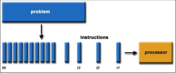
Traditionally, algorithms operate in a sequential fashion (Figure 1):
-
- A problem is broken into a discrete series of instructions
- Instructions are executed sequentially
- All instructions are executed on a single processor
- Only one instruction is executed at any moment in time
Multiple computing resources are utilized in parallel computing to solve a computational
problem simultaneously (Figure 2):
-
- A problem is broken into discrete parts that can be solved concurrently
- Each part is further broken down to a series of instructions
- Instructions from each part execute simultaneously on different processors
- An overall control/coordination mechanism is employed
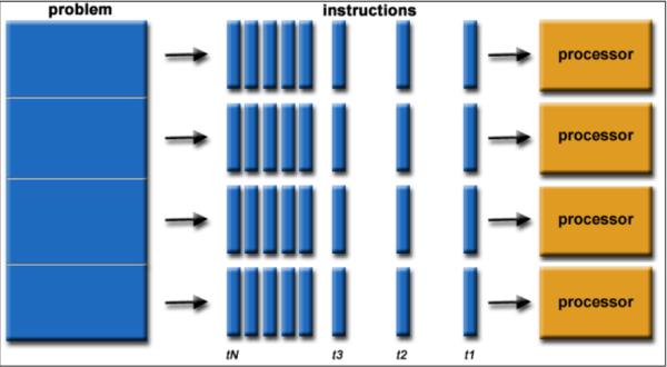
By dividing a task into X subtasks and executing them simultaneously, execution speed can be improved up to a factor of X times.
2.2. Distributed Computing
A distributed computing system is a hardware-software combination consisting of components that are located on different networked computers and communicate and coordinate actions among each other through passing messages. The components interact with one another in order to achieve common goals/tasks (Steen & Tanenbaum, 2017). A common distributed architecture is demonstrated in Figure 3:
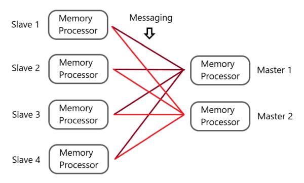
Each node in a distributed system consists of a memory component (RAM) and a processor component (CPU). The master nodes oversee distributing and managing data/tasks across the system, and slave nodes execute the tasks assigned to them by the master. The goal of a distributed system is to utilize all available memory and the processing power of different computers to solve a computational problem efficiently and in a fault-tolerant manner (i.e. evenif a few nodes fail, the system will continue to function).
2.3. Raspberry Pi
A Raspberry Pi (RPi) is a credit-card-sized, inexpensive single-board computer that is capable of running Linux and other lightweight operating systems based on ARM processors. An ARM processor belongs to a family of multi-core CPUs based on the RISC (reduced instruction set computer) architecture developed by Advanced RISC Machines (ARM). Figure 4 features a detailed description of the RPi 3 Model B+ components.
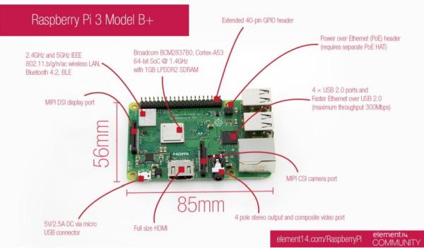
RPis, equipped with 1GB of RAM, a quad-core CPU at 1.4GHz, built on a robust motherboard, are used in this project. Each RPi is perfectly compatible with another RPi and thus, makes it easier to scale up just by adding more RPi units. After considering other options (i.e., Qualcomm DragonBoard, ASUS Tinker Boad, etc.) we decided that RPi was a suitable
choice for this project in terms of cost, functionality, portability, and scalability.
3. Building the system
3.1. Components and Costs
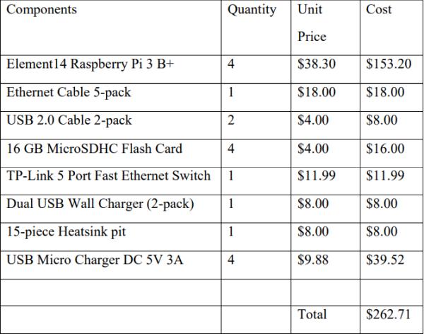
The total cost for this project is $262.71, which is detailed in table 1. We were able to use an existing monitor with HDMI-VGA cable, keyboard and mouse in the lab room, so there was no cost for those components.
Table 1: Components and Costs
3.2. General Architecture
The major components needed to build a computing cluster are:
-
-
-
-
-
- Computer hardware
- Operating System (OS)
- An MPI (Message Passing Interface) library
- An Ethernet switch
-
-
-
-
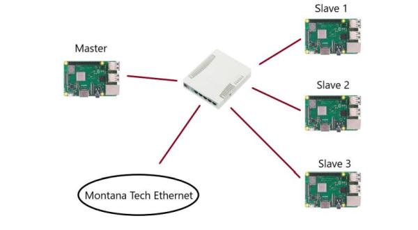
Figure 5 shows the main network architecture. The system design includes 4 RPi nodes, 5-port Ethernet switch, Raspbian OS, and MPICH with Python wrapper (MPI4PY). The RPis were connected to Montana Tech network through the Ethernet switch.
3.3. Operating System
For this project we considered two different operating systems for the Raspberry Pi: Raspbian and Arch Linux ARM. Raspbian is a Debian-based OS optimized for the RPi, which comes pre-installed with a full desktop environment and a large set of precompiled packages. For these reasons, Raspbian is great for getting started with RPi and Linux. The downside of using Raspbian is that it is bloated with many unnecessary packages leading to slower installation and start-up.
However, the Raspbian takes the fully-featured approach while Arch Linux ARM takes the minimalist approach. The default installation provides a bare-bone, minimal environment, which boots (in 10 seconds) to a command line interface (CLI) with the network support. With Arch Linux, the users can start with the cleanest, fastest setup and install only packages as needed, allowing the system to be optimized for different purposes (e.g. data processing, system administration, etc.). The disadvantage of Arch Linux is it has a much steeper learning curve for new users, who will have to manually install many packages and their dependencies using an unfamiliar CLI.
As the main goal of this project is to explore RPi, Linux, parallel and distributed computing, Raspbian was chosen for the OS for our system. Arch Linux may be considered for users more fluent in Linux operating system.
3.4. MPI and programming language
MPICH is a high performance and widely portable implementation of the MPI standard. We chose MPICH because it supports both synchronous and asynchronous message passing. Installation of MPICH and its Python wrapper (mpi4py) on RPi is also fast and simple. MPICH requires that all nodes have password-less Secure Shell (SSH) access to one another. We
achieved this by generating a pair of public-private keys for each node, and then copying the public keys of all nodes into each node’s list of authorized keys.
Python was an obvious choice of programing language due to its ubiquity in the scientific computing world and our own familiarity with the language. Python is especially suited for fast prototyping due to its syntax and the fact that it is interpreted and dynamically typed. Performance tradeoffs with Python include lack of type safety and slower execution time.
However Python was sufficient for the purpose of this project.
4. Testing the system
Once the system was built, we proceeded to test its basic functionality with a simple MPI program. Subsequently, we ran a Monte Carlo simulation in three different methods (sequential/parallel/distributed) and compare the performances among the methods.
4.1. Functionality testing
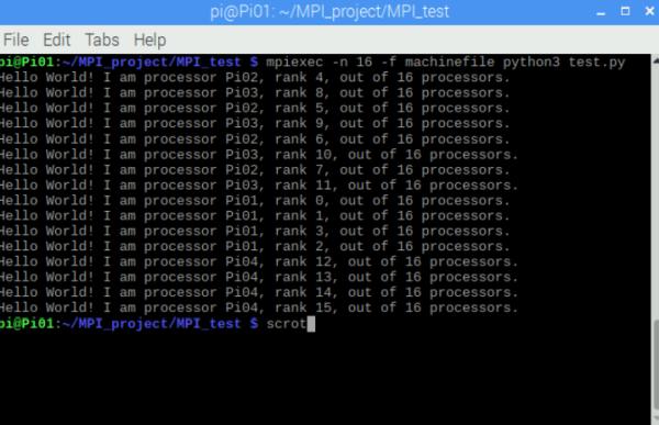
A simple “hello world” Python test script was sent by MPI from the master node to the slave nodes. Each of the 16 processor on the network needed to report back to the master to confirm that all of the processors were working correctly (Figure 6).
4.2. Monte Carlo approximation of Pi
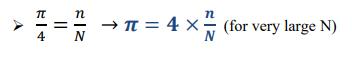
The Monte Carlo methods are a broad class of computational algorithms that rely on repeated random sampling to obtain numerical results. The essential idea in Monte Carlo methods is that randomness can be used to solve problems that might be deterministic in nature. In this project, we used a Monte Carlo algorithm to approximate the number π (Figure 7).
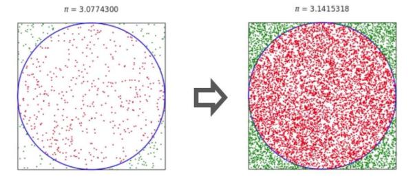
The steps are:
1. Generate a random point inside the unit square
2. Check if the point falls inside the circle enclosed by the unit square. Record the result.
3. Repeat steps 1 and 2 N times.
4. Count how many points fall in the circle enclosed by the unit square (n)
5. Calculate Pi by:
This algorithm is highly parallelizable because each point that is generated is completely independent of every other point.
4.2.1. Parallel Processing on a single RPi
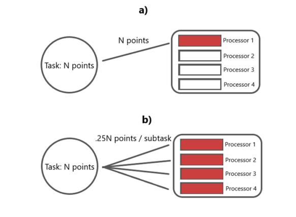
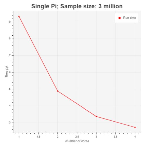
The second phase of testing was the Monte Carlo simulation. First, we ran the Monte Carlo algorithm with a sample size of 3 million in a sequential order meaning only 1 processor is involved in executing the task. Next, we used Python multiprocessing library to parallelize the task to 2, 3, and 4 subtasks, with each subtask being executed on a separate processor (or core) in a single node (Figure 8). In this case, the sample size was 3 million.
Prior to running the experiment, we expected that parallelization would greatly reduce the run time of the Monte Carlo algorithm, since the workload would be shared across multiple processors instead of a single processor. The results (Figure 9) confirm this expectation. A nearlinear improvement in run time was observed as more cores participated in sharing the workload.
4.2.2. Parallel vs Distributed Computing
After examining runtimes of sequential and parallel algorithms in a single node, we proceeded to explore the distribution of tasks and data across the network. First, we wanted to examine the effect of converting the data into TCP/IP format and sending them back and forth between the nodes in the network. Next, we distributed the task to all 16 nodes in the network to demonstrate the benefit of utilizing all available computing resources.
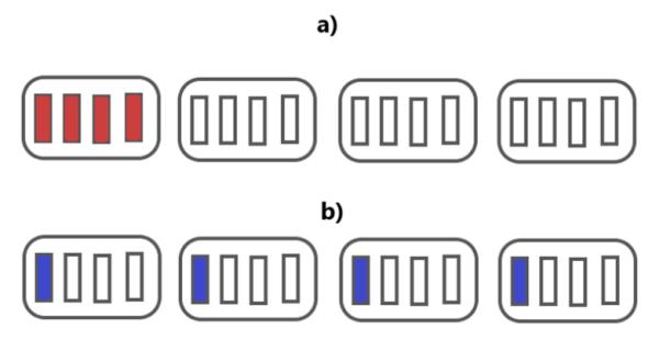
4.2.2.1. 4 cores: single node vs four nodes
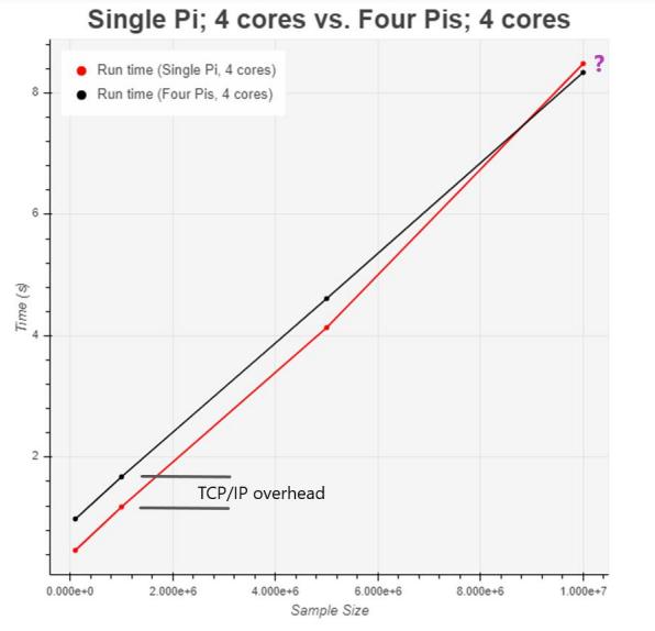
To examine the effect of data conversion and transfer, we divided a Monte Carlo simulation into 4 subtasks. Then we compared the performance of running 4 subtasks in a single node and of running 4 subtasks in four different nodes (Figure 10). The sample sizes that we used are 100 thousand, 1 million, 5 million, and 10 million.
The results are shown in Figure 11. For the first 3 data points, the results were as we expected. The overhead involved data conversion and transfer increased the runtime when we distributed the subtasks across the network. For the final simulation with sample size of 10 million, the results were surprising. Distributing the 4 subtasks across different nodes actually
outperformed processing the 4 subtasks in a single node. A likely explanation for this phenomenon is that for computationally-intensive tasks (e.g. large sample sizes), a single RPi would produce a lot of heat and slow down due to thermal throttling. This would no longer be the case if we distribute the subtasks across the network. Unfortunately, due to time constraints, we could not verify this hypothesis.
4.2.2.2. 16 cores vs 4 cores
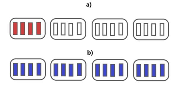
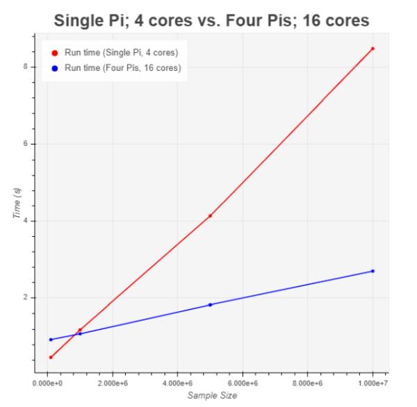
For the final experiment, the goal was to demonstrate the benefit of a fully distributed, fully parallel system where all computing resources were utilized. To achieve this, we compared the performance of running 16 subtasks across the network and 4 subtasks in a single node (Figure 12).
The results (Figure 13) show dramatic improvement in runtime when the other 3 nodes participated in sharing the workload. For a sample size of 10 million, run time was improved by almost a factor of 4.
4.3. Challenges encountered
The first problem we encountered was with installation of the software packages. Initially we tried to compile most packages from their source code, which was an extremely tedious and error-prone process. We had multiple compatibility issues due to missing dependencies, for which we had to completely reformat the SD cards and reinstall the operating systems. Later, we realized that we could use the Advanced Package Tool (APT) to install packages, which automatically installs in standard directories and takes care of dependencies. The only downside of using APT is a lack of customizability.
We also encountered another challenge with supplying enough power to the RPi. At first, our power sources could only deliver 1.1 A to each RPi, which was insufficient for running intensive computational tasks. Our master node kept rebooting whenever we attempted to execute a computationally-intensive task. We resolved this problem by using more powerful power sources that are capable of delivering 2.0~2.5 A to each RPi.
5. Conclusions
We successfully assembled and tested a 4-node computing cluster using Raspberry Pis. Using the cluster, we also demonstrated that parallelization and distribution of tasks and data are beneficial. Our cluster is a robust, low-cost distributed system that can be used for training and research activities in parallel and distributed computing.
In the future, we hope to scale up the system to hundreds of processors. In order to achieve this, we will need to design a physical structure that can house the RPis, and a method of delivering sufficient power to the system reliably. We will also consider optimizing this prototype by using a more compact operating system and/or a more performant programming
language.